A Full-Featured Open-Source Framework for Image Processing

Directional Blurs

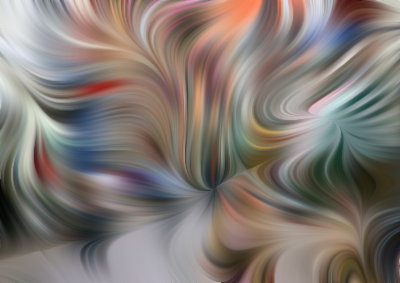
Lawdy. We've hardly messed with Cosine and Sine. Let's make corkscrews.

At first glance, it may not be clear how we went about setting EigenOne, EigenTwo, Cosine and Sine.

1.	For the eigenvalues, we started with a one pixel, two channel image with EigenOne set to constant one and EigenTwo set to constant zero. (1^0). We resized this to the input dimensions but did not bother to split the channels out as they are set to the way we would like to have them and are ready for -eigen2tensor.
2.	We made a tiny 5-by-5, two channel image for Cosine and Sine, using the special math notation 2*u-1. This sets the fifty or so pixels to random values between -1 and 1. u itself is an interesting variable, taking on a different value in the range of [0 – 1] every time it is referenced. We then resized this 5-by-5 image up to the dimensions of the input image, using a high quality cubic interpolation (go look at Ramp Recipes, which is where we got this technique).
3.	Whenever we use random processes we like to set the random number generator to a specific seed. Later, we can produce the exact same result. That's what -srand 78124 does. See plasma for details.
4.	orientation ensures that each pixel in our Cosine and Sine image are scaled to unit vectors.
5.	As with EigenOne and EigenTwo, there is no need to split out Cosine and Sine gray scales. We left them as two channel images ready for eigen2tensor.

In effect, we specified 25 random directions on a 5 by 5 grid. On resizing, we interpolated these samples over the much larger dimensions of the input image, using a cubic interpolation scheme. We got it by setting resize ’s interpolation parameter to 5. This filled the Cosine and Sine images with smoothly varying values for each pixel, these nestled among the original 25 explicit samples. The curves manifested by smooth are Bézier-like, which, like the interpolation used here, are grounded on cubic polynomials. Run this pipeline with other resize interpolation schemes and see what happens!

Zeroing Out EigenOne and EigenTwo

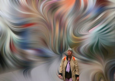
Despite utter chaos, some people Just Know How To Keep On Shopping.

We introduce a mask (msk.png) cut to the outline of the woman in the foreground. Nothing complicated. The woman is zero bits, everything else is 255. It sets a region in the EigenOne to zero. Concomitantly, EigenTwo is entirely zero, so the region occupied by our shopper has both EigenOne and EigenTwo set to zero, and she is not blurred at all.
So, generally, when both eigenvalues are zero blurring turns off.
And, more generally, we may vary the overall degree of blurring by varying EigenOne and EigenTwo. To the extent they differ, directional blurring take place.

Yea, yea, yea. We hear some of you out there telling us that all we had to do was select/float the woman off of a pristine copy and paste her onto the swirly stuff. Sure. No argument. Six of one. Half a dozen of the other. Either way, we're still cutting masks, and that's the time pig. Moreover, we're demonstrating principles here, and the principle here is: blurring is going to be no more than the larger of EigenOne or EigenTwo. Both zero. No Blur. That's the takeaway!

Selective Whirl Blur

Instead of total chaos, we can just have streamers of chaos.


The deal here is we took the luminance of the input image and then made a gray scale mask where the midtones map to white, but shadows and highlights map to black, the digerati's classic posterization curve.

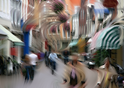
The tool for this is apply_curve, G'MIC's equivalent to GIMP's curve tool. We used this mask as a multiplier against EigenOne. EigenTwo is constant zero, so we are dealing with skinny blurring ellipses throughout. This gives rise to the hairlike swirl.
The effect is something like a selective blur, with the highlights and shadows holding structure while midtones form swirling banners.

The Anisotropic Smoothing Bits

We've been referencing the anisotropic smoothing bits for pages and pages without introducing them to you. That's because we live in Brooklyn, Noo Yawk and Why Do You Wanna Know?

OK. Got the Attitude out of the way. Here are the Anisotropic Smoothing Bits:

1.	structuretensors:	Finds edges. Makes a tensor field encoding where they are along with their orientation. Its output is often called a “structure tensor field” because the field encodes these edges and their orientations. This makes up the first part of the anisotropic smoothing pipeline. We rarely call structuretensors; smooth or diffusiontensors calls it on our behalf.
2.	diffusiontensors:	Calls structuretensors internally to perform edge detection and orientation, then finds the blurring directions and magnitudes for smooth. It encodes these in a “diffusion tensor field”.
3.	smooth:	The general purpose directional blurring tool. It's behavior is entirely dictated by the tensor map it is given. You can give it whatever you want. If you don't give it anything, anisotropic smoothing kicks in for the operand image. smooth calls diffusiontensors; diffusiontensors calls structuretensors and they pass tensor fields around. Eventually smooth gets a diffusion tensor field which tells it what to do.

At the data container level, diffusion and structure tensor fields look exactly the same. The conversion from structure to diffusion tensor fields entail redirecting and rescaling vectors, but one tensor field could easily be swapped for the other and smooth wouldn't care – it would just give you funny results and take a very long time to do it.

Along the way, there are two useful utilities.

1.	eigen:	Unpacks structure tensor fields into a set of vector magnitudes and directions – our EigenOne, EigenTwo, Cosine and Sine images. eigen packages these as a pair of two-channel images; we often further unpack them into four grayscale images. These are simple split and append exercises.
2.	eigen2tensor:	The functional reverse of eigen. Given a magnitude and direction pair of images, creates a tensor field. You can concoct your own magnitude and direction fields, as we have been doing throughout this Cookbook Recipe, then call eigen2tensor as a last step before invoking smooth.

---