A Full-Featured Open-Source Framework for Image Processing

Fake Depth Of Field

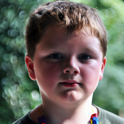"Photographier: c'est dans un même instant et en une fraction de seconde reconnaître un fait et l'organisation rigoureuse de formes perçues visuellement qui expriment et signifient ce fait." — Henri Cartier-Bresson

Henri Cartier-Bresson reminds us of the decisive moment when, in fleeting instances, the significance of events as well as their precise organization of forms, fall into place, giving the moments their proper expression.

Sometime later, my finger hits the shutter.

I suppose, with all the retouching that goes on, I'm not alone in this matter of moments missed nor with my collection of images off on one or another mark. This recipe deals with but one, that of an overly deep depth of field.

Depth of field is one of a number of framing devices toward which a photographer may reach, but it sits on a high shelf. One might stop up the lens for its wonderous framing along depth, but in the heat of the moment will the subject fall within just that apt focal plane? Struck with doubt, one goes for the high f-number, but a deep depth of field both increases the chance of capturing the subject and snaring Cousin Timothy picking his nose or Uncle Floyd scratching his butt. At least that how it goes in my family.

Ah, but there are times, opening a centennial birthday gift, when the explosion of joy on Great Aunt Matty's face is so precious that — one way or another — you must extract all but the lowest frequencies from the Floyds and Timothies of Camera Art and consign them to a Gaussian netherworld of indistinction, Great Aunt Matty's blurry backdrop.

This could be hard or easy depending on circumstances. We'll do easy, to demonstrate principles, then take on hard, which is how Life goes.

Jarrah Fence

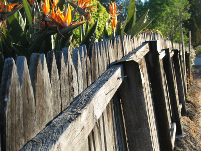Greg O'Beirne has given us a nice picture of an old jarrah picket fence in Western Australia. We fetched a copy from Wikimedia Commons. Around x = 740 → 820 there's a nail which we declare to be in the middle of our fake depth of field.

Our game opens with the synthesis of EigenOne and EigenTwo, which we duplicate. If you've been sticking with us since the beginning of these recipies, you'll recall that these two datasets manage blurring, and where these datasets are equal blur goes circular. In these circumstances, Cosine and Sine datasets become irrelevant — a circlular blur looks circular no matter how one tilts it. By habit, we set the Cosine gray scale to constant one and Sine to constant zero. That's an easy unit vector to remember and Cosine and Sine should, in the aggregate, hold unit vectors.

apply_curve is the bit that sets up EigenOne and EigenTwo — and the amount of blurring: black means 'no blur', white means 'blur lots'; downstream, -smooth's amplitude parameter, a multiplier, gives these expressions precise meaning. Concomitantly, -apply_curve is grounded upon a square graphical remapping relationship with x and y axes graduated from 0 to 255. X represents original intensities from the selected image; y indicates how these originals should change. Typically one explicitly sets around three or four pairs of x = have → y = want; G'MIC inbetweens the intermediaries. We conjure a prototype grayscale out of the aether and initially make it a left-to-right ramp. By itself, this protoype wholly blurs the right hand side but keeps the left pristine.

That's not quite our game, of course. However, the ramp essentially indexes left-to-right distances, associating a particular shade of gray, v, with a distance from the left hand edge of the image, x: v = 256x over w so, following conversion from distance to intensity, our have → want pairs become specifications of how much blurring we'd like to have at so many pixels out from the left hand side of the image. We want the nail at around x=740 to be sharp, i. e., "in (fake) focus", so the -apply_curve graph ought to map v = (256 × 740) ÷ 1280 ≈ 148 to a want value of zero. We'd like the left hand side of the fence the foreground slightly out of (fake) focus, perhaps, so maybe v = x = 0 maps to a want value of 63. Finally, we'd like the distant end of the fence to be deeply out of (fake) focus, so v = 255 mapping to a light gray want, 230 or so, pleases us very much. So our -apply_curve looks something like a lopsided V:

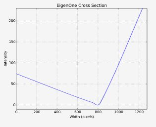
We think it is important to observe that none of these machinations have any basis in physical reality. The only (faint!) connection this jiggery has to reality is the mere fact that Greg O'Beirne set himself up by a jarrah fence so that one end of it was pretty close to the camera and the other end was pretty far, and, despite being nearly a century old, still ran more-or-less along a line, giving us something of a relationship of z-depth as a function of pixels in from the left hand edge of the image. Life is rarely so kind to us, as we will see in following example. When we said we'd do easy, this is easy. It will get worse.

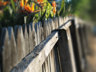We kick off three passes of -smooth at an amplitude of 200 and we're done. We drop the tensor field and write out a fake depth of field enhanced image.

That was easy. Harder to explain than do, but, as we noted before, this is a boundary case — we can fake a linear depth relationship between the horizontal position of pixels and their supposed distance from the camera because in this particular case, a fence plotted a line in three-space and the two-space relationship which assisted us was a projection of that line onto the picture plane. How nice! But most photographs will not present us with such ideal relationships. The big increment in complexity comes with those images where no clear relationship between pixel position and depth exists, and that is the majority of cases. Unless you've taken a stereo pair, or are producing images with a 3D modeler smart enough to give you a depth map, you will have to sleuth out how to paint the likes of EigenOne/EigenTwo. An example follows.

Moais of Easter Island

Artemio Urbina's Wikimedia Commons photograph of some of the 887 Moai on the island of Rapa Nui (Easter Island) illustrates a few of the typical issues arising from imposing a depth of field effect upon a photograph that is pretty much in focus throughout.

Setup

Broadly, it falls into your lot to approximate a depth map. It need not be too precise; indeed, it is usually impossible to be precise. The act of projecting a three dimensional space onto a two dimensional surface destroys information, in particular, depth information and judging depth becomes informed guess work. There are inherent ambiguities in such projections which Maurits Escher used to exploit with such charming regularity.

As with the Jarrah fence, our depth map task boils down to the synthesis of EigenOne and EigenTwo, giving each a gray scale image that establishes how much blurring will take place at each point in the image, which, in turn, is based on our guesses on how far three-space points are from the focal plane — itself a matter of guesswork. Unlike the Jarrah fence, we don't have an approximating formula; we compose the depth map by sherlocking, guessing and possibly tossing in a little pixel dust.

We may also have the additional chore of separating out into other layers regions of the image that fall into the putative focal plane. These regions will correspond to places where the image is "in (fake) focus." It is not sufficient to zero out EigenOne and EigenTwo areas corresponding to in-focus regions. At the end of the work stream there will be nothing more than a convolution kernel walking over an image, and unless we take preventative steps, when that convolution kernel is close to (but not in) a "no-blur zone" it will still factor in some of the pixel values from that no blur zone. This is especially true where a "no blur zone" abuts a "blur heavily zone," such as the moai's head (in focus) against the backdrop of the sky (very much out of focus). This gives rise to "halos" around the in-focus regions.

Our preventative steps entail lifting the objects we think are in the focal plane into a separate paint program layer, in a crude way restoring the depth information that the act of photographic projection had obliterated. This gives us a "front layer" and a "back layer". Pixels in the front layer are not convolved. Pixels in the back layer are — but first we repaint the back layer as if the foreground objects aren't there. Here are the particulars:

1.	cutting a mask,
2.	lifting the in-focus regions into a separate front layer, removing their pixels from all convolution operations that will run over the back layer, and
3.	Restoring regions in the back layer that had been occluded by front layer objects. This amounts to guessing what those regions looked like, and appropriately estimating their colors and luminosities so that the blurring around the foreground objects seem "correct."

We summarize the tasks here but leave out a lot of detail because particulars will vary. Your favorite paint program may not be mine, and we're documenting G'MIC here, not paint programs. That said, we cannot go into too much detail about the G'MIC pipeline because there is little detail to be had. The pipeline is virtually identical to the Jarrah fence example. The bulk of the work entails the mask cutting, isolating infocus regions, and backplane synthesis. Particulars, such as they are, follow. We have made bold filenames that will figure in the follow-on G'MIC pipeline.

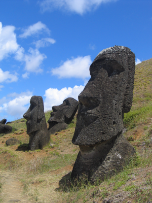	Moais on the flank of Rano Raraku at Rapa Nui (Easter Island), 2004. Artemio Urbina; Wikimedia Commons. Studying the image, every pixel seems in sharp focus. It seemed to be a very sunny day and we gather the lens was stopped way down. We decide that the moais are situated on a rising hillside, receding from a near point to the right out to a farpoint on the left. All this is guess work, but seems plausible. We decide that the near moai is in the focal plane, along with the strip of ground at its base and running diagonally up the hill. This decision, one of pure whimsy, establishes the black areas in EigenOne and EigenTwo. We declare by fiat that behind this "focal plane" a black-to-white ramp runs from right to left along the embankment. The point on the far horizon will be just off-white. The sky will be fully white as it is easily the deepest thing in this "depth map".
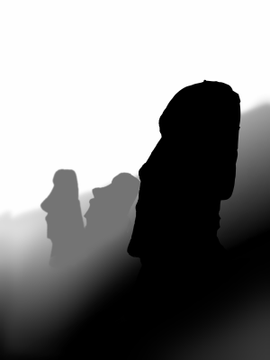	moai_depth.png After some thought, experimentation and guesstimation, we arrive at this "depth map" which may have some bearing on reality. This image serves as EigenOne and EigenTwo. Since, point-by-point, values in EigenOne equal EigenTwo, the overall blurring will be circular with the blurring ellipses at each point in the image varying only in size. The large moai right of center is black, a region which will not be blurred. The "depth map" seems like a still from a film noir production, but appearances can be deceiving. Paint programs are perfectly capable of saving RGB images that look like gray scales. EigenOne and EigenTwo, however, must be single channel images, otherwise the assembly of the tensor map will fail. Before saving moai_depth.png (or any depth map, for that matter), set the color mode to grayscale and remove the alpha channel.
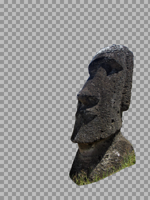	moai_focal.png Regardless of how we set values in EigenOne and EigenTwo, we must segregate objects in the "focal plane" to another layer. While the regions corresponding to the large moai are black in EigenOne and EigenTwo, and will be "in focus", there are adjacent regions which are not, and some – corresponding to the sky – will be quite light and subject to large circular convolution kernels that will reach into the neighboring moai and partially copy its dark pixels into the sky, creating a wholly unphotographic-like halo around the moai. A separation into layers needs to be considered wherever there are sharp discontinuities in the "depth map". We considered the middle ground moais as well, but decided that the effect would not be pronounced enough. Those moai are already being blurred somewhat, obscuring any halo effect that might surrond them. Mask cutting is time consuming, so we avoid it if at all possible.
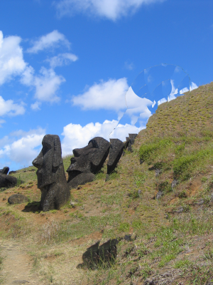	moai_backplate.png On the underlying layer we have synthesized grass-like and sky-like textures in the regions vacated by the moai, making the image as if the moai hadn't been there. At a very primitive level, convolution involves (partially) copying pixels. To maintain the fiction that grass and sky occupy the regions behind the vacated moai, we put grass and sky there in fact. With this, convolution will copy apt colors and values, minimizing halo effects. We are, of course, inpainting. We do not need the more sophisticated inpainting tools which have arrived with recent flavors of G'MIC. In fact, we used a simple cloning tool and worried little about repeat patterns or odd looking geometry. Afterall, in the regions we most care about, immediately around the edges of the vacated moai, there will be a fair amount of blurring going on, and the moai itself will bury many of our ghastly artifacts. What  we do care about, though, is matching tone and color, so we didn't clone grass where sky would be.

G'MIC Pipeline

Having constructed all the pieces we need in our favorite paint program, we do final assembly in G'MIC. G'MIC isn't playing as central a role as it normally does in these tutorials. The only reason we have a G'IMIC pipeline here at all is for its decent gradient blur. The preparatory work, making the depth field, cutting a mask and making a backplate, has dominated this workflow.

We trust that if you have reviewed the other recipes centered on the smooth command, the G'MIC script here should be familar, almost routine. We load the depth map, normalize and duplicate it, producing gray scale maps EigenOne and EigenTwo. The append command operating along the channel axis packages these gray scales into the scalar dataset that eigen2vector requires. Since these maps are pixelwise equal, the blurring ellipse will be circular throughout, so Cosine and Sine are irrelevant, but necessary, so we prepare a placeholder map; Cosine is a constant unit scalar, Sine is a constant zero scalar. Together they define a constant unit vector at each pixel oriented toward zero degrees. This is as good a placeholder as any. As is our wont, we scale these from single pixel images — the (1^0) notation. This produces the directional dataset that eigen2vector requires. With both datasets on the image list, we invoke eigen2tensor and that produces the tensor field. We apply the smooth command in the standard way that we having been using throughout: three passes at amplitude fifty. The smooth command often spreads a dataset over a slightly wider dynamic range than what the input image has. As a prudent matter, then, we normalize the output image into a range the paint program likes. Here, we used [0…255] that accommodates unsigned eight bit pixels.

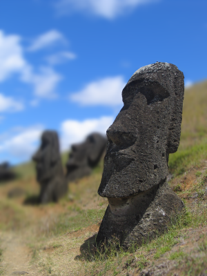With the graduated blur complete, we composited the large, righthand moai back into his old spot. We're done.

Postscript

Done well, our fake depth of field trick probably can fool some of the people all of the time. That is, if one reconstructs a spot-on depth map, exercises great care with the masks, and does a commendable job matching color and tone in the vacated areas of the backplate, there will be people who will think "What a nice/interesting/stupid/boring... photograph" without noticing the tooling marks ("Oh — the script kiddies are faking depth of field again.").

Chances are, photographers will notice the tooling marks. However, they may be too polite to mention anything. It is one of the extreme injustices of photojournalism that events do not repeat themselves. No matter how one pleads about the lens cap, Mount St. Helens is just not going to re-explode. So when Great Aunt Matty beams into that never-to-repeated look of joy, the working photographer knows that he or she will need to deal with Floyd and Timothy and, having used such necessary fakery herself, is hardly going to complain when it is used by others.

That said, they still know better. Contrary to our usual wont, the frontpiece to this recipe is not a bit of G'MIC gimmickry, but a straight forward picture of a young boy inhabiting a narrow depth of field. Compare the blurs of the frontpiece image with the "out-of-focus" Jarrah fence.

T'ain't the same.

How lenses distribute light is only (very approximately!) gaussian. Observe the bokeh pattern on the lefthand side of the frontpiece image. Some of the edges are quite abrupt; not at all like the continuous change in color and tone which characterizes -smooth. Bokeh is only one among many phenomena which occur as light passes through a lens assembly.

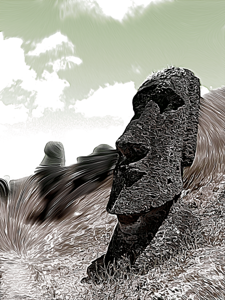
Aptly enough, there is a fuzzy line between photojournalism and photographic illustration, such that there are those who delight in the "unreality" of computer-generated depth of field. For those who care to walk that line, then the equality between EigenOne and EigenTwo may very well be one of the first things that the photo illustrator abandons, along with constant Cosines and Sines. We leave you with an uncommented example, something of a visual summary of this sequence of cook book recipes on doing your own diffusion tensor field.

---