 Home
Home Download
 News
News Mastodon
 Bluesky
 X
X Summary - 17 Years
 Summary - 16 Years
 Summary - 15 Years
 Summary - 13 Years
 Summary - 11 Years
 Summary - 10 Years
 Resources
 Technical Reference
 Scripting Tutorial
 Video Tutorials
 Wiki Pages
 Image Gallery
 Color Presets
 Using libgmic
 G'MIC Online
 Community
 Discussion Forum (Pixls.us)
 GimpChat
 IRC
IRC Report Issue
| Table of Contents ▸ Managing 3D Vector Objects | ◀ Installing the G'MIC-Qt Plug-in For 8bf Hosts | Scientific Publications ▶ |
Managing 3D Vector Objects
G'MIC is able to create, manage and display 3D vector objects. Although it may be considered as a minor feature for an image processing framework, it has in fact many implications in the way new commands can be developed, even for applying effects on usual 2D images.We describe here the various aspects of this interesting feature.
1. In which case do I encounter 3D vector objects ?
Basically, 3D vector objects in G'MIC can be generated from one of these sources :1.1. Reading a file (.off, .cimg[z] or .gmz formats)
For now, there are very few file formats storing 3D vector objects that G'MIC is capable of loading/saving:.off files: this is the format used by Geomview, a simple 3D object viewer available for Linux. This format stores the object data (vertices, primitives, colors..) as simple ascii text. This format is not able to store textured primitives, nor image sprites.
.cimg[z] and .gmz files: this is the native image format defined by the CImg Library that underlies G'MIC, to store generic image data, including 3D vector objects.
Here is a simple example of loading a 3D vector object, and displaying it with the command line tool gmic of G'MIC:
$ gmic caesar-40k.off
[gmic]-0./ Start G'MIC parser.
[gmic]-0./ Input 3D object 'caesar-40k.off' at position [0] (21627 vertices, 42622 primitives).
[gmic]-1./ Display 3D object [0] = 'caesar-40k.off' (21627 vertices, 42622 primitives).
[gmic]-1./ Selected 3D pose = [ 320,0,0,0,0,320,0,0,0,0,320,0,0,0,0,1 ].
[gmic]-1./ End G'MIC parser.
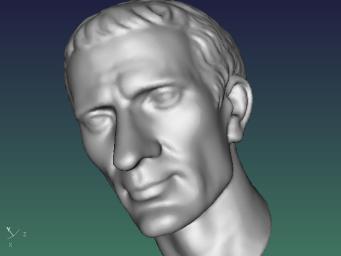
Fig. 1: Example of visualizing a 3D vector object .off file, by the G'MIC integrated 3D viewer.
1.2. Extracting a 3D object as an image feature
G'MIC has some commands to transform/extract/convert features of regular images as 3D vector objects. For instance, the command imagecube3d creates a 3D cube where the elected image has been mapped on each of the 6 faces of the cube.Command elevation3d generates a 3D vector object that represents a 3D elevation of the selected image, as shown below:
$ gmic lena.bmp rs ,128 blur 2 elevation3d 0.2
[gmic]-0./ Start G'MIC parser.
[gmic]-0./ Input file 'lena.bmp' at position [0] (1 image 512x512x1x3).
[gmic]-1./ Resize 2D image [0] to 128 pixels along the Y-axis, preserving 2D ratio.
[gmic]-1./ Blur image [0], with standard deviation 2, neumann boundary and quasi-gaussian kernel.
[gmic]-1./ Build 3D elevation of image [0], with elevation factor 0.2.
[gmic]-1./ Display 3D object [0] = 'lena.bmp*' (16384 vertices, 16129 primitives).
[gmic]-1./ Selected 3D pose = [ 2.51969,0,0,-160,0,2.51969,0,-160,0,0,2.51969,-119.103,0,0,0,1 ].
[gmic]-1./ End G'MIC parser.
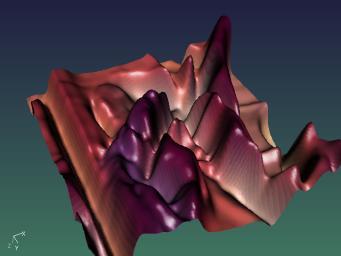
Fig. 2: Example of 3D object, obtained as an elevation of a regular 2D color image.
1.3. Generating 3D objects from scratch
Some other commands are able to generate 3D vector objects "from scratch", without needing additional image data. For instance, commands torus3d or circles3d are able to do that:$ gmic torus3d 100,20 sphere3d 30 +3d
[gmic]-0./ Start G'MIC parser.
[gmic]-0./ Input 3D torus, with radii (100,20) and subdivisions (24,12).
[gmic]-1./ Input 3D sphere, with radius 30 and 3 recursions.
[gmic]-2./ Merge 3D objects [0,1].
[gmic]-1./ Display 3D object [0] = '[3D torus]*' (930 vertices, 1568 primitives).
[gmic]-1./ Selected 3D pose = [ 1.26106,0.416099,0.119812,0,-0.331563,0.690643,1.09126,0,0.278495,-1.06191,0.756682,0,0,0,-294,1 ].
[gmic]-1./ End G'MIC parser.
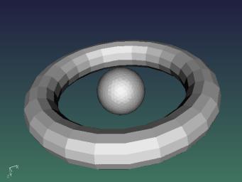
Fig. 3: Example of 3D object, generated from scratch by using G'MIC commands.
Look at the 3D Meshes section of the reference documentation to see all available commands to create 3D objects from images or from scratch.
2. How 3D vector objects are internally stored.
2.1. Why should I care about this ?
In G'MIC, a 3D vector object is stored as a regular image. The only thing is, this kind of images has a special structure (image size and ordering of pixel values) that makes it recognizable as a 3D vector object, by the G'MIC interpreter. As a consequence, anyone can write custom commands able to generate 3D objects, as such objects are not different than any other image. Knowing this allows to quickly create complex 3D objects, for instance without having to use explicit loops (which are bottlenecks for performances in many interpreted languages). As 3D objects can be drawn into images (with command object3d), it becomes also interesting to use them instead of using loops even for dealing with 2D images. We will show an application of the use of 3D objects to create a custom (and fast!) version of the histogram command afterwards.2.2. The different parts of a 3D vector object.
What makes a 3D object data recognizable from an usual image ?First, it is stored as one-column scalar image, with dimensions 1xNx1x1 (where N is usually very big). Then, they are basically vectors which contains all the necessary informations to entirely define a 3D vector object.
These informations appear in this order, to define the 3D object features :
A magic number, to make a 3D vector object easily recognizable regarding other one-column images. It is unlikely that a random vector will start with this serie of numbers.
The numbers of vertices and primitives that are composing the 3D object.
The list of vertices coordinates (x,y,z).
The list of primitives (type and structure).
The definition of the colors/textures for each primitive.
The definition of the opacity/masks for each primitive.
Each of these 6 parts composing the whole 3D vector object are detailed below.
Before going further, one has to notice that the command split3d is exactly able to split any 3D object into 6 different images that correspond to these different parts of the object. Using it on an existing 3D object is a really interesting way to do some reverse engineering of the data structure, and see how the object has been encoded as different parts in a one-column image:
$ gmic box3d 100 split3d display append y
2.1. Magic numbers
The magic numbers define a sequence of 6 numbers which represent a header for recognizing an image as a 3D vector objects in G'MIC. These numbers are actually the ASCII codes of the string CImg3d, eventually with a float-valued part (usually, 0.5 is added to each of the ASCII values for being even more random and unlikely to appear in real image data). To get the exact values for these ASCII codes, you can use G'MIC of course :)$ gmic echo "{'CImg3d'}"
[gmic]./ Start G'MIC interpreter (v.4.0.1).
67,73,109,103,51,100
[gmic]./ End G'MIC interpreter.
[gmic]./ Start G'MIC interpreter (v.4.0.1).
67,73,109,103,51,100
[gmic]./ End G'MIC interpreter.
which means that the magic sequence of numbers is
67,73,109,103,51,100
(+epsilon, with 0<=epsilon<1).
An one-column image which starts with these values is likely to be a 3D vector object in G'MIC. But, it is not sufficient. The remaining object data must have a valid structure too. If only one of the data is missing or incorrectly structured, the image will not be seen as a 3D vector object, but as a regular image instead.
Be aware that there is a very strict checking of the image structure to determine whether an image represents a 3D vector object or not.
2.2. Number of vertices and primitives
A 3D vector object is basically composed of :A set of 3D vertices, each with coordinates (x,y,z).
A set of primitives. Each primitive references the indices of the vertices that are a part of the primitive.
So, the number of vertices (V) and primitives (P) are two global variables that are mandatory to define a 3D vector object. These two values appear in the image data just after the sequence of magic numbers.
2.3. Vertices data
Each vertex of a 3D vector object is represented by a triplet (x,y,z).The vertices data are then stored as the sequence of the three coordinates (xi,yi,zi), for i from 0 to V-1. These coordinates can be anything you want, as they are float-valued. They don't have to be bounded.
2.4. Primitives properties
That's the more complex part of a 3D vector object, as primitives can be defined in a very flexible way. They may have different shapes (dots, segments, filled triangles, with or without textures, etc...). So the difficulty is one primitive will be defined by a sequence of values which size depends on the type of the primitive to encode.The first value N of a primitive sequence represents at the same time, the type of the primitive, and the size of the encoding.
A primitive is then described by a sequence of N+1 values.
Depending on the first value N, the next encoding values have different meanings :
If N==1 : The primitive is a colored point (or a sprite image). The next value is the single indice of the corresponding vertex.
If N==2 : The primitive is a colored segment. The two next values are the indices of the two vertices composing the segment.
If N==3 : The primitive is a colored triangle. The three next values are the indices of the three vertices composing the triangle.
If N==4 : The primitive is a colored quadrangle. The four next values are the indices of the fours vertices composing the quadrangle.
If N==5 : The primitive is a colored (perfect) sphere. Perfect here means that the sphere will be drawn using a filled circle, and is not composed of triangulated faces. The two next values are the indices of the two vertices that defines one diameter of the sphere. Next value can be { 0=filled sphere | 1=outlined sphere}. Other two next values are ignored.
If N==6 : The primitive is a textured segment. The two next values are the indices of the two vertices composing the segment. Then, the next values are (xt0,yt0,xt1,yt1), the texture coordinates of the two vertices of the segment.
If N==9 : The primitive is a textured triangle. The three next values are the indices of the three vertices composing the triangle. Then, the next values are (xt0,yt0,xt1,yt1,xt2,yt2), the texture coordinates of the three vertices of the triangle.
If N==12 : The primitive is a textured quadrangle. The four next values are the indices of the fours vertices composing the quadrangle. Then, the next values are (xt0,yt0,xt1,yt1,xt2,yt2,xt3,yt3), the texture coordinates of the four vertices of the quadrangle.
2.5. Primitives materials
Just after the definition of the primitive types comes the definition of the primitives materials (color or texture data). As for the definition of primitives structures, the material of each primitive can be encoded with a variable number of values.The sequence of numbers defining a primitive material can be:
Either (R,G,B), the RGB color of the primitive (applies for primitives with N=1,2,3,4 or 5).
Or, the magic sequence (-128,W,H,S,d0,d1,..,dM) that defines an image data associated to the primitive (texture for instance). The material image is then a 2D multi-spectral image of size W x H x 1 x S, filled with pixel data d0,d1,...,dM, where M=WxHxS-1.
It can be used to associate a texture to a primitive (applies for primitives with N=6,9 or 12), or an image sprite to a pointwise primitive (N=1), or to define a color primitive that may have more than 3 channels (for N=1,2,3,4 or 5).Sometimes, it is desirable to define several 3D primitives which share the same texture, but with different texture mapping coordinates. In that case, providing a data copy of the same texture for each primitive would be cumbersome. That's why it is possible to define a material image that is shared with another primitive instead, using the magic sequence (-128,ind,0,0), where ind is the indice of the primitive with whom the texture is shared (this primitive can itself share his texture if needed).
That way, there are several possibilities to define primitive materials.
2.6. Opacities
Then, comes the definition of the primitives opacities. It is pretty close to the way materials are defined. Each primitive opacity can be defined by :Either (O), a single float value that defines the opacity of the primitive. O==0 means the primitive is fully transparent, O==1 means it is fully opaque, and O==-1 means it is additive.
Or, the magic sequence (-128,W,H,S,d0,d1,..,dM) that defines an image data associated to the opacity (useful to define sprite masking, for pointwise primitives N=1). It works the same as for the primitives materials, with the possibility to have shared opacity masks as well.
2.7. Putting all this together
Now, you know how to define every part of a 3D vector object in G'MIC.Once again, remember that command split3d is able to decompose an existing 3D objects as a set of these 6 property vectors.
To generate a 3D vector object from all these 6 property vectors, just append them along the y axis, with command append y.
The example below shows how we can write a command that create a 3D vector object from scratch, without having to use anything else than input expressions :
my_3dobject :
({'CImg3d'}) + 0.5 # Magick numbers.
(7,6) # 7 vertices, 6 primitives.
(-1,-1,0,\ # Vertice [0]
1,-1,0,\ # Vertice [1]
1,1,0,\ # Vertice [2]
-1,1,0,\ # Vertice [3]
0,0,0,\ # Vertice [4]
0,0,-1,\ # Vertice [5]
0,0,1) # Vertice [6]
(4,0,1,2,3,\ # Primitive [0] = colored quadrangle.
5,4,6,0,0,0,\ # Primitive [1] = colored (perfect) sphere.
2,0,5,\ # Primitive [2] = colored segment.
2,1,5,\ # Primitive [3] = colored segment.
2,2,5,\ # Primitive [4] = colored segment.
2,3,5) # Primitive [5] = colored segment.
(255,0,255,\ # Color primitive [0] = magenta.
0,255,0,\ # Color primitive [1] = green.
255,255,255,\ # Color primitive [2] = white
255,255,255,\ # Color primitive [3] = white
255,255,255,\ # Color primitive [4] = white
255,255,255) # Color primitive [5] = white
(0.6,1,1,1,1,1) # Opacities are all 1 except for quadrangle.
unroll y a y # Merge all the features as single 3D vector object.
and then
$ gmic my_3dobject
will generate this object: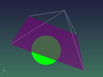
Note that the command below would generate almost the same 3D object, and is definitely more comprehensive and easy to code:
my_3dobject2 :
circle3d 0,0,0.5,0.5 col3d[-1] 0,255,0
quadrangle3d -1,-1,0,1,-1,0,1,1,0,-1,1,0 col3d[-1] 255,0,255 o3d[-1] 0.6
line3d 0,0,-1,-1,-1,0 line3d 0,0,-1,1,-1,0
line3d 0,0,-1,1,1,0 line3d 0,0,-1,-1,1,0
col3d[-4--1] 255,255,255 +3d
circle3d 0,0,0.5,0.5 col3d[-1] 0,255,0
quadrangle3d -1,-1,0,1,-1,0,1,1,0,-1,1,0 col3d[-1] 255,0,255 o3d[-1] 0.6
line3d 0,0,-1,-1,-1,0 line3d 0,0,-1,1,-1,0
line3d 0,0,-1,1,1,0 line3d 0,0,-1,-1,1,0
col3d[-4--1] 255,255,255 +3d
But in the latter case, each primitive will be merged independently, without sharing any vertices, so at the end, the object generated by my_object3d2 will be bigger (14 vertices) than the one generated by my_object3d (7 vertices).
So, generating your own 3D objects using the internal structure coding is not mandatory, unless you have good reasons to do so. It demands some efforts, and often the vector image we obtain do not comply with the very strict memory structure of a 3D vector object (one byte missing is enough to make it not recognized as a 3D vector object!).
A good way of understanding where the problems are coming from is to try forcing display the 3D object, with command display3d (shortcut: d3d). When this command fails, it outputs a quite descriptive error message that helps to understand the issue.
In the next sections, we show an example on how it can be useful sometimes.
3. Using 3D vector objects to speed up 2D image processing
One of the nice thing with 3D vector objects in G'MIC is that they can be drawn on regular images, using command object3d. And of course, to be fast enough, this drawing command is a native one, and to draw the 3D object, it loops over the list of all primitives and draw them at their 2D locations (that are the projections of the 3D coordinates regarding the orientation of the 3D object).That means that the object3d command is able to quickly draw generic primitives (points, segments, ...) on quite random locations of a 2D image. This characteristic of the command can be advantageously used to replace usual loops in some G'MIC commands.
It may be sounds a bit tricky (and it is), but this often allows to speed up the execution of a command surprisingly.
We show here a simple example that code a simpler version of the histogram command, with an usual loop, and with the use of 3D vector objects.
3.1. Computing an histogram: the naive way
Challenge : Suppose you have one input image with integer values in [0,255], which I want to compute the histogram of, and of course without using the histogram command.A quite naive way of doing this would be :
my_histogram :
i[0] 256 # Create the target histogram
repeat h y=$>
repeat w x=$>
val={i($x,$y)}
=[0] {$val+1},$val
done
done
i[0] 256 # Create the target histogram
repeat h y=$>
repeat w x=$>
val={i($x,$y)}
=[0] {$val+1},$val
done
done
If we call this command, and see how long it takes (lena.bmp is a 512x512 scalar image):
$ time gmic sp lena my_histogram print quit
[gmic]-0./ Start G'MIC parser.
[gmic]-0./ Input file 'lena.bmp' at position [0] (1 image 512x512x1x3).
[gmic]-2./ Display images [0,1] = '[unnamed]*, hist'.
[0] = '[unnamed]':
size = (256,1,1,1) [1024 b].
data = (0,0,0,0,0,0,0,0,0,0,0,0,... 0,0,0,0,0,0,0,0,0,0,0,0) [float].
min = 0, max = 3177, mean = 1024, std = 955.111, coords_min = (0,0,0,0), coords_max = (149,0,0,0).
[1] = 'hist':
size = (512,512,1,1) [1024 Kio].
data = (156,156,156,155,156,151,157,155,158,155,156,154,...75,79,82,88,98,95,100,107,103,106,107,109) [float].
min = 38, max = 227, mean = 123.173, std = 41.1275, coords_min = (508,71,0,0), coords_max = (117,272,0,0).
[gmic]-2./ End G'MIC parser.
real 0m30.183s
user 0m29.958s
sys 0m0.064s
It works as expected (as it gives the same result as histogram actually), but it is painfully slow because of the two nested loops over the image pixels that are interpreted again and again (no, G'MIC has not JIT compiler !)
3.2. Computating an histogram: using 3D objects tricks.
Now, what if we decide to use 3D vector objects in our histogram computation commands ?Basically, the idea would be to consider that each pixel value i(x,y) of the original image should be drawn as a point (with additive opacity) onto the target image (histogram), at position X=i(x,y). Looks like the problem of histogram computation can be see as the drawing of a 1d point cloud on an initially black image.
A 1d point cloud can be obviously declared as a 3D vector object, where each primitive is a single colored point (with value 1), and each primitive opacity is set to -1 (additive drawing).
So here we go :
my_histogram2 :
i[0] ({'CImg3d'}) # 3D object magick number.
i[1] ({w*h*d*s},{w*h*d*s}) # Number of vertices / primitives.
unroll[2] y columns[-1] 0,2 # Vertices coordinates in 3D : (X,0,0)
1,{h},1,1,1 1,{h},1,1,y a[-2,-1] x # Associate point primitive to each vertex.
3,{h},1,1,1 # Primitives colors.
1,{h},1,1,-1 # Primitive opacities.
unroll[-6--1] y a[-6--1] y # Merge as a 3D vector object
256 object3d[-1] [-2],0,0,0,1,0,0,0 # Draw into target histogram
rm[-2]
And now, we get :
$ time gmic sp lena my_histogram2 print quit
[gmic]-0./ Start G'MIC parser.
[gmic]-0./ Input file 'lena.bmp' at position [0] (1 image 512x512x1x3).
[0] = '[unnamed]':
size = (256,1,1,1) [1024 b].
data = (0,0,0,0,0,0,0,0,0,0,0,0,... 0,0,0,0,0,0,0,0,0,0,0,0) [float].
min = 0, max = 3177, mean = 1024, std = 955.111, coords_min = (0,0,0,0), coords_max = 149,0,0,0).
[gmic]-1./ Quit G'MIC instance.
real 0m0.947s
user 0m0.804s
sys 0m0.136s
We avoided loops in our code, making them internally executed by the object3d command, and the gain of time spent is impressive, as we are 3000% faster now !
That is a typical example where it is interesting to know how 3D vector objects are internally stored in memory, as we can generate them to speed up our algorithms.
Actually, lots of existing G'MIC custom commands are using this kind of technique : grid, pointcloud, display_polar, distribution3d, and so on...
Conclusions
G'MIC defines a very flexible way to deal with 3D vector objects, as anyone can generate them from scratch (sometimes this may require a lot of efforts!).For advanced G'MIC programmers, knowing how to generate these objects by ordering the object data correctly in memory will allow them to optimize their custom commands.
Probably not for used everyday, but it can greatly optimize your G'MIC scripts. Definitely one of the trickiest thing to know about the G'MIC script language, but a powerful way to gain computational time !