Tiled Art
 | Mosaics are an ancient medium. Examples date back to the third century B.C., but the form is still active, employing materials from seashells to bottle caps. It recruits orientation itself to its services. Artists align tiles with dominant edges, lending these greater clarity. Other ranks follow, and from dominant edges wavefronts ripple outward and – inevitably – collide. Work is cut out for the mosaic artist who must carefully chip compromises all along the collision fronts. Interesting work if you can get it. Image: Mosaic of Justinianus I - Basilica San Vitale (Ravenna) Wikimedia Commons: Petar Milošević |
 | 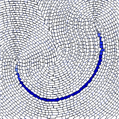 |
| Old Stroke | A Tiled Old Stroke |
Introduction
The demonstration command gtutor_tileit illustrates a technique of G'MIC vector drawing whose behavior is conditional on the features found in a bitmap "guide image". Given dominant edges detected in the bitmap, orient vector-drawn tiles to those edges, in a manner similar to traditional mosaic tiling techniques. This walkthrough is based on a simplifed version of gtutor_tileit. Postscript goes into the differences.Orienting tiles along dominant edges is but one kind of surface tessellation. Strictly speaking, the technique outlined here does not tesselate, as coverage is rarely complete. Collision fronts and rank mismatches almost always give rise to gaps. Mosaic artists keep various kinds of workarounds in their kits, from breaking regular tiles into irregular shapes and daubing extra plaster in the less significant holes.
That said, the technique here is not without mathematical interest. Edge detection and orientation have been in G'MIC's kit for a long time, part and parcel with edge-preserving smoothing.
The game is straightforward:
| 1. | First, find some edges. |
| 2. | Harness distance to establish measures from arbitrary points to edges. |
| 3. | Harness gradient to establish their two-dimensional orientations. |
| 4. | Try not to plot too much. |
| 5. | But also try to plot where we should with centerlines and orientaton angles to tell us how. |
| 6. | From these data, derive affine transformation matrices to translate, scale and rotate the corners of a reference tile, situated at the origin, to placements situated in the mosaic. |
| 7. | Render the placed tiles. |
| 8. | Probably there will be missed spots. We punt. |
Here's our play.
Edges
Step 6 embodies the heart of it: translating, scaling and rotating tiles according to the orientation of nearby edges. First – we have to find edges. To that end, the technique uses a very simple forward differencing scheme to elucidate "important" edges – that is, the ones we notice. Faint edges thankfully escape attention as mosaics orienting toward too many edges appear jumbled.With dominant edges located, -distance and -gradient determine how far image points are from edges and how tiles laid on top of them should align. These commands have tutorials elsewhere; only summary treatments reside here.
 | 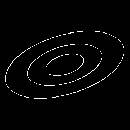 |
| flat color | edges of same |
| 1. | Locate edges Edge, distance and orientation data stem from image -luminance, so single channel images convey the essential ideas. A straightforward contour detector from Jerome Boulanger locates the important edges. It forward differs the leading and lower diagonal pixels of a 3 × 3 grid against a candidate situated at grid center. As a forward differencing scheme, no heed need be paid to top, bottom and rear quadrants. Of the forward quadrants, only southeast and due east differences matter. The northeast pixel is taken care of, as it is also the due east pixel in the next most northerly pass. That is, in a left-to-right, top-to-bottom in-place fill, it has already been set. Two tests suffice: |
-fill. ">abs(
i-j(1,1,0,0,0,1) # Southeast edge?
)>iv?
1: # Yes, otherwise...
abs(
i-j(1,0,0,0,0,1) # East edge?
)>iv?
1:0" # Yes, otherwise no edge.
-name[-1] outline # Outline: basis of distance calculation
i-j(1,1,0,0,0,1) # Southeast edge?
)>iv?
1: # Yes, otherwise...
abs(
i-j(1,0,0,0,0,1) # East edge?
)>iv?
1:0" # Yes, otherwise no edge.
-name[-1] outline # Outline: basis of distance calculation
| The test thresholds against overall image variance, a heuristic choice. A forward difference less than this fails to be "interesting enough" for orienting tiles along it. |
What Is That Mess after the -fill Command?
It is a Pixel Processor.Pixel and Pel Processors
-fill, -eval and -input all take string parameters constituting math expressions. Such math expressions implicitly operate on all pixels in the command's selection decorator in a particular traversal order. Its remit is to produce a pixel – in "vector" mode – or, in "scalar" mode, a single-channel pixel component called a pel.Depending on its mode, the processor replaces the former pixel entirely (vector mode) or one of its component pels (scalar mode). How this happens follows entirely from the math expression's coding. The final computation becomes the replacement value, an implicit assignment from the expression to the pixel or pel. The form of the replacement value sets the mode, vector or scalar. Simply, returning scalar values puts the processor in scalar mode; returning entire pixels — vectors, realized as numeric lists in square brackets — puts the processor in vector mode.
The pixel processor can do whatever it wants to compute the replacement value — accessing, in any manner, the current or neighboring values, values in other images, or values entirely uncoupled from any image, such as the special random number generating value u. Here is a one character pixel processor based on u:
-input 128,128,1,3,u -normalize. 0,255 # An image filled with random values.
Edge Detection
The edge detector here is encoded using the conditional ternary operator, which has three parts: <condition> ? <expression-then> [: <expression-else> ] The third part is optional, signified by the square brackets (do not use the square brackets when actually writing a conditional ternary operator).| 1. | The condition is composed around a logical relationship and is required. A ? marks its end. Here, the condition expression for the edge detector is abs(i-j(1,1,0,0,0,1))>iv and asks "is the absolute difference between the current pel (i), and its southeast neighbor ( -j(1,1,0,0,0,1) ) greater than the prevailing image variance?" |
| 2. | The expression-then executes if condition is true; expression-then is required. It may be followed by a colon, and should this be the case the optional expression-else follows. For the edge detector, expression-then is simply a return value, the scalar 1 (the processor is in scalar mode). A difference greater than the overall image variance is taken to mean the presence of an edge to the southeast of the center pixel, causing the center pixel to be set by expression-then — simply 1. Testing is complete when the condition is true; expression-else, if it exists, does not execute. |
| 3. | A colon : separates the optional expression-else. It executes only if condition is false. |
For the edge detector, expression-else is a second conditional ternary operator that operates as the first - but testing the center against the due east pixel instead. This is an example of cascading ternary operators so as to successively test other possible conditions; these may run to any number of stages, but the edge detector only needs two tests: "variance straight ahead" and "variance to the southeast". Here, if there is a large variance straight ahead, then the center pixel is set to scalar 1. Otherwise, it is set to 0. Thus, if both forward differencing tests fails, then the center pixel is set to zero indicating that no edge is present in the forward direction at a one pixel radius. Should one or the other succeed, then the center pixel is set to one, indicating an edge.
Examining the Neighborhood
We have left much out of the picture. For example, the j() function is intended to sample the neighborhood around the current pixel upon which the processor operates (a pixel at position [ x, y ] with the value i ). For generality, j()'s first four parameters are [ dx, dy, dz, dc ], relative coordinates with respect to the current pixel. These can be fractional, pemitting subpixel sampling of the neighborhood around the current pixel. With sub pixel sampling, one may also choose the kind of interpolation through the fifth parameter: 0 for nearest pixel, 1 for linear interpolation or 2 for cubic interpolation. The sixth and last parameter chooses a boundary policy. See Images Have Edges: Now What? for the necessity of choosing what to do when close to image edges. Here, 0 asserts the policy that "imaginary" pixels beyond actual image edges are to be regarded as black (Dirichlet policy). 1 asserts that such "imaginary" pixels just continue the values of their nearest "real" edge pixel along the column or row (Neumann policy). 2 asserts a Periodic policy: "imaginary" pixel values arise from joining the near edges with far, as if the flat image is rolled into a doughnut shape. 3 asserts Mirror policy. "imaginary" pixels beyond the edge by a delta distance have the same value as that of a "real" pixel just the same delta from the edge.Traversal Order
The edge detector's design embodies a particular traversal order: pixels are to be examined in a left-to-right, top-to-bottom traversal. Should the opposite traversal take place, the conditional tests may not work properly.When it is necessary to specify traversal order, math expressions will place a particular interpretation on the initial character of the expression, which can set the traversal order. Here, a leading > character sets left-to-right, top-to-bottom traversal; note that the edge detector expression begins with this character. On the other hand, < sets a right-to-left, bottom-to-top traversal. Both traversal orders operate in place. As the processor proceeds, it overwrites old values with new; presumably, it has no need to refer to overwritten values anymore. Both traversal orders use only one thread, which may disappoint those with multi-core CPU's.
To engage other cores, omit > and <. G'MIC then analyzes the pixel processor and, if it can, parallelize the code across cores. In this case, it is not possible to depend on any particular traversal order as any number of independent threads operate on the image asynchronously. Clearly, this is a condition in which the edge detector cannot operate, but many math expressions are agnostic about traversal order. If such a case holds, then leaving out the traversal leading character can speed up math expression a great deal.
Conversely, one may force parallelization by using : – multithreaded and in place or * – multithread on an image copy and transfer the result to the image. Demanding multithreaded operation may not actually speed up the pixel processor. Experiment and prepare for disappointment.
Further Information
The edge detector harnesses just these math expression elements: a particular traversal order, neighborhood sampling (i, j()) and testing based on the conditional ternary operators. There is a good deal more to math expressions; see the technical reference Mathematical Expressions for expression syntax, standard functions, coding rules and math expression conventions.Distance and Orientation
Edges begat distances and orientations, the direct antecedents to placing oriented tiles.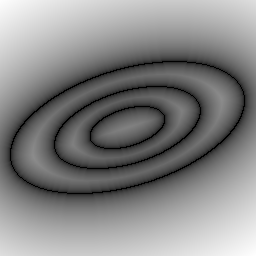 | 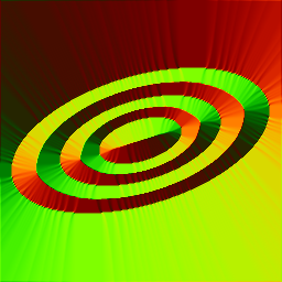 |
| distance | orientation |
| 2. | Distance and Orientation From edges, distance and orientation follow directly via the distance and gradient commands. The target isovalue, 1 for distance measuring, is just the boolean output value of the edge detector. Pixels with this value necessarily map to zero, as an isovalue is always at measure zero from itself. All other pixels map to their Euclidean distances to the nearest edge. Orientation follows readily from distance by pairwise differencing from pixel to pixel along both x and y axes, estimating a gain or loss of "height" at the pixel of measure – the remit of the gradient command. The normalization of these data obtains vectors of magnitude one which span the lines of steepest gradients toward edges. The two channels of the orientaton image contain the sines and cosines of these directions, directly indicating how much to rotate the tile to align with the gradient. |
-distance[outline] 1 # Make Euclidean metric to edges
-name. distance
+gradient[distance] xy
-append[-2,-1] c
-orientation[-1] # Alignment vectors with respect to edges
-name. orientation
-name. distance
+gradient[distance] xy
-append[-2,-1] c
-orientation[-1] # Alignment vectors with respect to edges
-name. orientation
Culling
In principle, enough is known now for tile-laying, but practical considerations intrude. We are not contemplating laying down a tile at every point in the image, are we? Seems excessive, so a culling scheme is in order.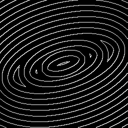 |  |
| centerlines | orientation |
| 3. | Culling Of the ways to write image-filling expressions, the single-threaded, fill-in-place variant suggests itself, set through an initial > math expression character. Fill-in-place means that the results of a mathematical expression replace pixels as they go along. With this behavior, and with a candidate plot point in hand, we determine if the candidate pixel has already been tiled; we do not plot again in such a case. Thus, so long as we fill-in-place, the act of plotting tiles itself culls: no plotting of tiles until the traversal reaches a candidate that has not already been tiled. This scheme supposes that the "plotting field" is preset with "sentry pixels", so-called because the pixel vector cannot possibly be a product of tile rendering. We might create a plotting field filled with [-1], perhaps, and tile only with positive values. But by what means do we identify "candidate plot points"? From the ideas that tiles have common heights and centerlines stems a notion of periodic markings radiating from identified edges. Apart from other considerations, we plot only when we have a candidate point on a tile "centerline". Where do centerlines come from? Employing round, we convert distance measure to a staircase, with the width of the step corresponding to tile height and step-to-step changes corresponding to centerlines. Edge detecting the value changes gives centerlines: a [1] marker in a field that is otherwise [0]. |
# Centerlines from distance
-round[distance] {$tsz}
-fill[distance] ">
abs(i-j(1,1,0,0,0,1))>"{0.5*$tsz}"?
1:
abs(i-j(1,0,0,0,0,1))>"{0.5*$tsz}"?
1:0
"
-name. centerlines
Here $tsz is an command line input variable that represents "tile size"; it has been derived from a command line parameter or is a default tile size; we need not worry too much about which is which. For purposes here, it sets the height of the tile, which, through rounding, has been equated to change of pixel intensity. Apart from the different test value, this centerline detector is virtually the same as the edge detector used before. When the fill completes, the old distance image converts to a centerline chart.-round[distance] {$tsz}
-fill[distance] ">
abs(i-j(1,1,0,0,0,1))>"{0.5*$tsz}"?
1:
abs(i-j(1,0,0,0,0,1))>"{0.5*$tsz}"?
1:0
"
-name. centerlines
Plotting
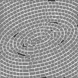
At this juncture, we have two of the necessary images already enlisted: one depicting the centerlines and the other orientations. We initialize the third, plottingfield, by way of -input through dimension specifications and fill it with the sentry value: [-1]. # Plotting field:
-input [-1],[-1],1,1,'[-1]'
-name. plottingfield
-input [-1],[-1],1,1,'[-1]'
-name. plottingfield
The gist of conditional logic comes down to this: plot tiles on centerlines where no tile has yet been plotted – the candidate is on a centerline [1] pixel in the centerlines image and on a "never-been-tiled" pixel [-1] in the plottingfield image. As these pixels reside in different images, our conditional logic has to "span" those images — that is, reference pixels in both centerlines and plottingfield. In addition to that, we need to reference orientations to learn how to position a tile once we settle on the path to lay down a tile.
Referencing Various images in Math Expressions
Math expressions would be quite inflexible if their scopes were limited to just the image being filled. Expression scope can extend to every image on the list through index decorators. To each of the standard constants the math expression parser associates with images an index decorator can be appended. The decorator begins with a hashmark (#), optionally, a sign follows and the decorator concludes with a ordinal number. The ordinal number selects an image from the list; a negative sign indexes the ordinal number from the end of the list. The absence of a sign infers indexing from the start of the list, just as in selector decorators. Thus ia#-2 is the average value of the second image from the end of the image list and w#1 is the width of the second image from the beginning of the list — recall that image lists start at zero, in case you think our counting is off!
The notation extends to the image neighborhood sampling functions: i(x,y,0,0) reports the value of a pel at the current position, slice zero, channel zero. i(#0,x,y,0,0) reports the same value specifically from the first image on the list. If, in a pixel processor, we read some <condition> as 0<i#-3 && i#-1==-1 then a True evaluation arises if the current pixel value in the third image from the end of the list is greater than zero, AND to current pixel value in the last image on the list is negative one, a condition we test for in the following pseudocode.
Pseudocodingly, let us traverse plottingfield from left-to-right, top-to-bottom, and for each position [ x, y ]:
| 1. | reference centerlines. if the current pixel is on a center line, and |
| 2. | reference plottingfield. if the current pixel has not already been tiled |
| 3. | then |
| a. | transform tile corner points from reference to plotting positions using the sine and cosine values from the orientation image |
| b. | plot the tile using the math expression function polygon(). |
 |  |  |
| centerlines | orientation | plottingfield |
-fill[plottingfield] ">if(
0<i#-3 && i#-1==-1, # Plot tile?
xfrm=eye(3); # Compose Affine Matrix
xfrm[0]=I#-2[1];
xfrm[1]=I#-2[0];
xfrm[2]=x;
xfrm[3]=-I#-2[0];
xfrm[4]=I#-2[1];
xfrm[5]=y;
tl=xfrm*[-"$tsz", "$tsz"/2.0,1]; # Apply Affine Matrix
tr=xfrm*[ "$tsz", "$tsz"/2.0,1]; # to tile corners
bl=xfrm*[-"$tsz",-"$tsz"/2.0,1];
br=xfrm*[ "$tsz",-"$tsz"/2.0,1];
polygon(#-1,5, # Tile fill
[tl[0],tl[1]],
[tr[0],tr[1]],
[br[0],br[1]],
[bl[0],bl[1]],
[tl[0],tl[1]],
1,[127]);
polygon(#-1,-5, # Tile outline
[tl[0],tl[1]],
[tr[0],tr[1]],
[br[0],br[1]],
[bl[0],bl[1]],
[tl[0],tl[1]],
1,0xffffffff,[255]);
i,i)" # Double 'i'? See Postscript
| 4. | Plotting The -fill command, selects pottingfield and conditionally renders tiles to that image. The command takes a math expression pixel processor that consists of one if(<condition>,<expression-then>,<expression-else>) statement. Here is how it plays out: |
| a. | The <condition> embodies pseudocode steps 1. and 2. The first test, 0<i#-3 reflects step 1. It tests if the current pixel in centerlines is greater than zero. Should that hold, the current pixel is on a centerline. |
| b. | If the first test holds, then the second test, i#-1==-1 plays, reflecting step 2. This tests if the current pixel in plottingfield still retains the sentry value, [-1]. that is, it tests if a tile isn't already covering the location. |
| c. | Should either test fail, then <expression-else> executes at the end of the expression; it simply reasserts the current value of the pel, i. |
| d. | Should both tests succeed, then the bulk of the expression, the embodiment of <expression-then>, executes. <expression-then> does four things: |
| i. | create an affine transformation matrix, xfrm, to tranform tile corner points, |
| ii. | translates those points. from reference positions to corner plotting points in plottingfield. |
| iii. | uses those points to fill a tile rectangle, via the math expression polygon() |
| iv. | uses those same points to draw the tile rectangle outline, again using polygon(). |
| e. | An affine transformation matrix allows the encoding of two dimensional rotations, scalings and translations in one 3 × 3 matrix. To pull this trick off, we hold that two-dimensional points and lines on a surface are projections of analogous three-dimensional objects: A surface point at [ x, y ] has an analogous space point situated at [ x, y, 1 ]. To use the affine transformation matrix, we operate on the three dimensional space points and their two dimensional shadows follow along. |
Affine Spaces and Transforms
When it comes to rendering, a strictly two-dimensional point of view is limiting. A 2 × 2 transformation matrix embodies scalings and rotations — or compositions of both. The matrix cannot directly accommodate translations; in a strictly two-dimensional setting, we translate by adding displacement vectors, [ dx, dy ] to locations, a separate operation.
The notion of a displacement vector also suffers from a certain ambiguity with respect to points. Does a thing with two coordinates, [ x, y ], denote a position at the given coordinates? Or is it a vector oriented by the coordinates? Such ambiguity, and the limited purview of two-dimensional matrices, gives rise to an idea regarding two dimensional points and vectors as projections of three dimensional analogs.
With this point of view, a two dimensional point [x, y ] shadows an analogous object situated at [ x, y, 1 ]. The game is: do the transformations in three dimensions and the two dimensional shadows follow along.
With this approach, useful bookkeeping happens: subtracting two homogeneous points, [ a, b, 1 ] and [ k, j, 1 ] yields the vector that points from the second to the first: [ a – k, b - j, 0 ]. As a consequence of the differencing operaton the results has a third coordinate equal to zero and, in this extended notation, can be taken as a distinguishing characteristic of vectors. On the other hand, a third coordinate of one distinguishes points. In this fashion, the ambiguity between vectors and points falls away.
In this approach, adding points is meaningless; the third coordinate becomes two. What, after all, is the aim of adding two points? If one's aim is to model a displacement, then that may be best accomplished through the addition of a displacement vector to a point: the result of such an operation is the second point displaced from the first by a vector. In this operation the third coordinate of the result is one, reflecting that the results of this point-vector sum is the displaced point. Broadly, this point of view provides - and enforces - certain systematic operations between points and vectors, constituting an affine space. Such a space is defined on a set of points and the vectors reflecting possible displacements among those points. It is a space in which we can perform operations on points and vectors and obtain clear results.

| 5. | The first part of the <expression-then> assembles an affine transformation from the pixel in orientation at [x, y]. The channel values of this pixel, you recall, are the sine and cosine values that permit us to orient the tile along the gradient and the nearby edge. The x y coordinates themselves furnish the translation portion. Overall, the transformation matrix translates and aligns "template points," [a, b, 1], composing an origin-centered reference image of a tile, over to [j, k, 1] representing points that draw the tile in plottingfield. xfrm represents the affine transformation matrix in the math expression. We transcribe the current position and the sine and cosine trigonometrics from orientation to this matrix, compute the plotting locations of tile corners, then plot the image twice: first to fill, and then to delineate tile edges. And so we go onto the next [x, y] position and evaluate again. And so forth. And so on. Until we have traversed the image. |
 |  |
| plottingfield | diagnostics |
Punting
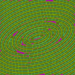
Of course we miss spots. And this is by intention. We didn't want an ideal tesselator; we wanted a tesselation that imitates a mosaic artist's (lack of) diligence. So when we test if a spot is "free and clear" to place a tile, we simply look for a center point, without regard to determining whether other tiles are in the bounding box. Such leads to overlap.Alternatively, we detect a tile — just barely! — and fail to make a placement in a space that is almost big enough. diagnostics shows holes with a purple shade. In gtutor_tileit, we furnish the user with a fillholes switch to establish the final disposition of holes: treat them as tiles, or furnish an alpha channel and poke a hole in it; the user does some post-processing compositing, perhaps to show an underlying wall.
Postscript
gtutor_tileit
This walkthrough is a simplification of the demonstration command gtutor_tileit. Much was dropped in the simplification in the interest of staying with the key idea: demonstrate some G'MIC vector drawing that is conditional on features found in a bitmap image.Differences are:
| 1. | Disruption: We obtain that by introducing noise to distance, which shows up in orientation, imparting additional twists to tiles. |
| 2. | Spread: This is a tile height multiplier that directly contracts or spreads centerlines. One may spread or, alternately, overlap, tiles. |
| 3. | Lighting: Same as that used in Fingerpaint. gtutor_tileit switch fcolor (flat color) disables fingerpaint lighting. |
Double i's in -fill[plottingfield]? How Come?
3. Math expression functions constitutes G'MIC's foray into structured vector drawing, akin to Inkscape. That said, the command processor still expects math expressions to return some kind of value for the current pixel (vector mode) or pel (scalar mode). Accordingly, the last statement in <expression-then> is simply i, returning the current pixel value.Astute readers may recall that one of the triggers in <condition> is i#-1==-1; that is, the drawing of the tile is a consequence of i being -1 in plottingfield. So doesn't this final statement in <expression-then> disrupt tile drawing? Won't it plot a -1 pel in the center of the tile? That is the value of i, no?
By a kind of G'MIC sleigh-of-hand, no; a subtle consequence of in-place rendering. With the initial evaluation of <condition>, the value of the current pel can indeed be -1 triggering tile drawing as a constituent operation of <condition-then>; subsequent tile-drawing by calls to polygon() alters i in place, its former value of -1 overridden. With the last statement of <condition-then> i has assumed its new value.
One may easily imagine other circumstances where i should retain an atomic persistence; that it shouldn't change in medias res. That is not the providence of an in-place traversal scheme. If persistence of original pixel and pel values matter to <condition> testing, then a traversal scheme other than in-place is in order. In this case, our culling strategy depends on an in-place change of the sentry value, -1 by the wholesale rendering of tiles with positive pel values. This chameleon-like behavior of i is a feature for us, not a bug. Other times, other cases, and we should keep in our kits that conditional testing like if(<condition>,<expression-then>,<expression-else>) should not heedlessly be taken as atomic operations.


 Home
Home Download
 News
News Mastodon
 Bluesky
 X
X Summary - 17 Years
 Summary - 16 Years
 Summary - 15 Years
 Summary - 13 Years
 Summary - 11 Years
 Summary - 10 Years
 Resources
 Technical Reference
 Scripting Tutorial
 Video Tutorials
 Wiki Pages
 Image Gallery
 Color Presets
 Using libgmic
 G'MIC Online
 Community
 Discussion Forum (Pixls.us)
 GimpChat
 IRC
IRC Report Issue