 Home
Home Download
 News
News Mastodon
 Bluesky
 X
X Summary - 17 Years
 Summary - 16 Years
 Summary - 15 Years
 Summary - 13 Years
 Summary - 11 Years
 Summary - 10 Years
 Resources
 Technical Reference
 Scripting Tutorial
 Video Tutorials
 Wiki Pages
 Image Gallery
 Color Presets
 Using libgmic
 G'MIC Online
 Community
 Discussion Forum (Pixls.us)
 GimpChat
 IRC
IRC Report Issue
fill (f)

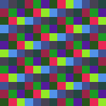
Newton-Raphson Weeds: This is why your trial root sometimes goes off into the rough
Filling Stuff
You have an image and wish to fill it with something. If you are new to G'MIC and coming from a paint program like GIMP, then your first thought after encountering this command might possibly be: “Ah HA! the fill command! At last I can fill circles and squares and things with red!”Well yes. And no. If paint buckets come to mind, then go over to fill_color, next aisle down, the one labeled Color Manipulation. That’s OK. Lots of people get lost in here first time through. G'MIC is a big place.
That isn’t to say you can’t use fill to make an image red. It’s just that you will have do it with a little finesse:
gmic input 2,2,1,3 fill. 220,220,220,220,20,20,20,20,60,60,60,60
This gives you an image filled with red:
X11 Crimson
The command’s numeric parameters inject a carefully arranged data stream into a freshly minted 2 X 2 pixel, single slice, three channel image. The data are so arranged as to fill this tiny image with the X-11 color Crimson: 0xdc143c, or decimal: 220, 20, 60. The individual numeric elements take their seats in the target image by first filling channel zero, row zero, starting at column zero, then going to column one, then two and so on. You have to arrange your data stream in a
like manner; fill doesn’t know about any other ordering schemes.
G'MIC geeks may find this excessively verbose, preferring:
gmic '(220,220;220,220^20,20;20,20^60,60;60,60)'
This also gives you an image filled with red:
Even More X11 Crimson
This G'MIC expression is terser, but dispenses with fill entirely. Instead, the second example implicitly invokes the input command. The input specification to which that command adheres uses commas, semicolons, carets, slashes and parentheses to describe image topology. This makes the terser example somewhat more informative at a glance.
However, since fill is the topic of this tutorial and we maintain a sentimental attachment to our tutorial topics, we’ll just send those interested in terse efficiency over to the aisle marked "Input-Output". They’re having a blue-plate special on input streams today. fill itself does not use input 's file specification. Its world-view is limited to ordered, one dimensional streams.
You may gather from this that fill is a fairly low-level command. Indeed. It fills images with pels. That’s it.
Pel, you ask? Pel is shorthand for Picture Element, an indivisible quantum of an image. Could be a byte long. Could be longer. Could even be shorter. Might be a float, or an unsigned integer – or even a signed integer. The particulars of a pel's organization stems from the image format.
But a pel is not a pixel. Pixels are vector-like and have components. On the other hand, pels are scalars, Pixels are assembled from pels. Pels are components of pixels. Careless scriveners may write ‘pixel’ when they mean ‘pel’ but we make the distinction here because the essential item that fill manipulates are pels. An RGBA pixel has four pels, and, we should note, fill could touch upon that particular kind of pixel as many as four distinct times while filling an image. At its most basic, then, fill pours pels into
images from some notional stream.
The notional stream can be specified in three ways:
Pel Streams: A literal stream of numbers – pels – that is the form we have discussed so far.
Images: Another image already on the list – same approach, really, but the pels have been packaged as an image instead of a literal sequence.
Math Expressions: A formula. Specifically, a pel generator derived from a G'MIC math expression.
This last notional stream is really quite an interesting way. Instead of draining pels from an input, a G'MIC math expression executes, producing the requisite pel. This processor has access to the pel's former value, or the pixel it inhabits, or the image containing the pixel, or the G'MIC image list holding the image, and the processor can access any of these data sources in any order – or none of them at all. With a math expression, you can do pretty much do what you want.
PEL Streams
The easiest streaming method to grasp is probably not the most practical – though there are exceptions to this. You can just stream comma-separated pels into an image, an open-ended argument list.Notice that, in contrast to the image specification streams used by input, there are no structure markers – No opening or closing parentheses, commas do not denote columns – they just separate pels, the semicolons that separate successive columns into rows, the carets which separate a plane of rows into channels, the slashes which separate a series of channels into slices – none of those appear in fill arguments. Nada. Ziltch. They aren’t needed. Images already have a built-in structure of slices, channels, rows and columns. fill just – well – fills them, following the topology of the target image.
In light of this, order your data stream according to the dimensions of the target image.
1. The largest (implicit) divisions in the pel stream are image slices. The fill command fills the first slice of a selected image entirely before starting on the second and subsequent slices, should they exist.
2. Within a slice, fill populates channel zero completely before beginning on channel one and subsequent channels, if they exist.
3. Within a channel, fill populates the top image row completely before the second and subsequent rows.
4. Finally, fill populates rows from column zero through to column w – 1, with w, the width of the image.
So you block out your data first by slices, within slices by channels, within channels, by rows. As a consequence of this, the pels that make up a multi-channel pixel are separated by a stride. For an image in the RGB color space, the red component is in channel zero. w×h pels downstream comes the green component. w×h pels further downstream comes the blue component. Revisit our initial example, above, for a tiny stride example.
Data streams need not be properly sized, which gives rise to a class of pattern generation. If fill runs out of a source stream while there is still space left in the target image, it starts at the beginning of the source stream again. fill loops over streams as many times as is necessary to fill a particular image. Once the target image is filled, the command discards the remaining excess.
So to make any one of a bazillion or so herringbone patterns, have some fun with discrete math and clock arithmetic:
![input 20,20,1,3 fill. 205,127,63,91,31,16,8 resize 150,150,[-1],[-1],1 normalize. 0,255](img/input_20_20_1_3_fill_205_127_63_91_31_16_8_resize_150_150_1_1_1_normalize_0_255.png)
Basic herringbone
gmic \
input 20,20,1,3 \
fill. 205,127,63,91,31,16,8 \
resize. 150,150,[-1],[-1],1 \
output. herr_00.png
input 20,20,1,3 \
fill. 205,127,63,91,31,16,8 \
resize. 150,150,[-1],[-1],1 \
output. herr_00.png
![input 17,17,1,3 fill. 189,129,6,207,84,104,239,153,6,78,85 resize. 150,150,[-1],[-1],5 normalize 0,255](img/input_17_17_1_3_fill_189_129_6_207_84_104_239_153_6_78_85_resize_150_150_1_1_5_normalize_0_255.png)
Herringbone soft
gmic \
input 17,17,1,3 \
fill. 189,129,6,207,84,104,239,153,6,78,85 \
resize. 150,150,[-1],[-1],5 \
normalize 0,65355 \
output. herr_01.png
input 17,17,1,3 \
fill. 189,129,6,207,84,104,239,153,6,78,85 \
resize. 150,150,[-1],[-1],5 \
normalize 0,65355 \
output. herr_01.png
Tweak the numbers following the fill command. Add a few. Take a few away. The game is to choose pel streams with lengths that do not evenly divide the capacity of selected images, or which do not evenly divide various image dimensions. Pel streams with lengths equal to prime numbers furnish a never-ending source of delight, should it be your wont for that kind of herringbone pattern.
In these examples, we use resize with different interpolation schemes to upscale and filter the herringbone pattern for additional effect. In the last example, we re-normalize the image immediately before output to ensure that the pels range within the limits imposed by the 16 bit/channel Portable Network Graphics format, since the cubic interpolation scheme we specified for resize can carry values outside this range. See Images As Datasets elsewhere on this site for a discussion on why this step is sometimes necessary.
Images
The fill command can populate one image with the contents of another. Instead of a stream of pels, we pass an image selection parameter in square brackets. The images in the selection becomes the fill source; Targets live in the selector decorator adorning the fill command.Beware: fill is not a cheap version of array. The command effectively flattens the source into a one dimensional stream of pels. The very first pel in the source stream corresponds to column zero, row zero, channel zero of slice zero of the target image. The fill command then increments, first by columns, then by rows, then channels, then slices, following the same hierarchy it imposes on literal pel streams. Indeed, as far as fill is concerned, an image is just a convenient way to specify a pel stream. Unless the source and target images happen to have identical dimensions, fill will not preserve image coherency. For that, investigate array.
This notwithstanding, we can still play herringbone games by building a herringbone pattern in stages:
![13,13,1,3 fill. 65,71,36,154,27,84,39,233,146,82 256,256,1,3 fill. [-2] o. img/big_herringbone.png o.. img/small_herringbone.png](img/_13_13_1_3_fill_65_71_36_154_27_84_39_233_146_82_256_256_1_3_fill_2_o_img_big_herringbone_png_o_img_small_herringbone_png.png)
big_herringbone.png
gmic \
input 13,13,1,3 \
fill. 65,71,36,154,27,84,39,233,146,82 \
input 256,256,1,3 \
fill. [-2] \
output. big_herringbone.png \
output.. small_herringbone.png
input 13,13,1,3 \
fill. 65,71,36,154,27,84,39,233,146,82 \
input 256,256,1,3 \
fill. [-2] \
output. big_herringbone.png \
output.. small_herringbone.png
small_herringbone.png
This example illustrates using fill with a pel stream, making an initial small herringbone image using a hand-written pel stream, then making a large herringbone using the initial pattern as an image source.
Fill Pitfalls
Here is an example you don’t want to do – unless you are being devious.
face.png

face times four
When the selected target image has dimensions 144 X 144, the fill command will not make a 2 X 2 array of four 72 X 72 happy faces. That is, instead of the image above, the commands:
gmic \
input face.png \
input 144,144,1,4 \
fill. [-2] \
output funny.png
input face.png \
input 144,144,1,4 \
fill. [-2] \
output funny.png
produces this strange image:
Funny faces
We’ve heard it said that fill is a low-level command. It just streams pels into an image. That's really all it does. Essentially fill turns source images into pel streams. Thus, the four channel, 72 X 72 happy face becomes a linear stream of 82,944 pels. Having flattened its source image, fill then populates its selected 144 X 144 X 1 X 4 target image using the precise same hierarchy we stated before: it completely fills the first slice of the target before commencing the second, and within a slice, it completely fills channel zero before commencing on channel one, and so on.
In particular, the fill command took the first 72 pel row of channel 0 of the source image and filled just the left half of the first row of the target image, which is, at 144 pels, twice as long. The second 72 pel row of the source image now fills the right half of the first target row. And so on. That explains the pair of flattened happy faces: the left half of the target image consists of the even rows; the right half contains the odd rows of the source image.
One quarter of the way toward filling the target’s channel zero, the source channel zero taps out. No matter. The fill command just begins streaming in the source’s second channel, copying those second channel pels into the target’s still not entirely filled first channel. Since the dimensions of the target image are exactly twice that of the source, with the area of each target channel exactly four times that of the source, the entire happy face source image exactly fills just channel zero of the target. The source has been entirely used up. Still no matter. The fill command goes back to the beginning of its source and commences to fill channel one of the target image through a second pass of the source.
At the end of the day, the source image is copied four times, each time filling just one channel of the target. That makes the four channels of the target image exact duplicates – hence, the target image is a study in gray of flattened happy faces. Could be they are not that happy.
The fill command is not a blitter – a block copier. It does not think in rectangles, just streams. To do what you really want to do, try array instead:
gmic
input face.png
array. 2,2,2
output. face-times-four.png
input face.png
array. 2,2,2
output. face-times-four.png
Math Expressions
The third way to stream pels is really quite different. The source – well, there is hardly a source in the literal sense. The source is what an algorithm encoded in a math expression produces when given a pel. The math expression is a pel processor written in G’MIC’s math scripting language.fill, along with its cousin input, both furnish hooks for pel processors, enabling fine-grained computations at the pel level. When the G'MIC command processor discovers that fill has been given a math expression as an argument, it suspends its own processing and invokes the math expression parser. That math expression now sources a virtual stream of pels. It is invoked once for every pel in the target image and the expression can do whatever it wants to produce that pel - accessing in any manner the current or neighboring pels in the target image, pels in other images on the list, or none of these sources at all, as in the first example following, which simply pulls random numbers out of the ether without regard to the content of the target or any other image on the list. The final computation of the math expression, whatever that result may be, becomes the new value of the pel, an implicit assignment.
Here are a few examples:

1967 Color TV
gmic \
input 300,300,1,3 \
fill. 'u' \
normalize. 0,'{2^8-1}' \
output colortv.png
input 300,300,1,3 \
fill. 'u' \
normalize. 0,'{2^8-1}' \
output colortv.png
The pel processor is one character, u, which is a math expression hooks into a random number generator. It’s invoked 300 x 300 x 3 = 270,000 times, once for each pel in the image. On each invocation, it produces a random value between the limits zero and one inclusive. Since this is the last computation this processor performs (as well as its first), G’MIC implicitly assigns the resulting random value to the pel. A one character script and you’ve written a generator that emulates a 1967 color television set tuned between stations. I bet if you thought about it for any length of time, you’d wind up writing a much more involved script for this very same VFX, assuming you wanted such a thing.

Bendexter
gmic \
input 300,300,1,1 \
fill. 'x==y' \
normalize. 0,'{2^8-1}' \
output bendexter.png
input 300,300,1,1 \
fill. 'x==y' \
normalize. 0,'{2^8-1}' \
output bendexter.png
Draws a one pixel bend dexter. Pels on the diagonal have equal column and row coordinates, so, for those elements, the math expression returns 1 (True: white), otherwise it returns 0 (False: black). That is, the pel is set with the boolean result of the comparison. Without further commands, the dynamic range of the image is from zero to one, which may not be what you want, so normalize the image for eight {2^8-1} or sixteen {2^16-1} bit precision, as suits.
x and y are two of many predefined variables available to math expressions, these providing the current pel's column (x) and row (y) coordinates. Similarly, there are current slice (z) and channel (c) coordinates that are predefined, while i furnishes the value of the pel addressed by (x, y, z, c).
Variable names in the GMIC Handbook furnishes a complete listing.

bendsinister
gmic \
input 300,300,1,1 \
fill. x==h-y \
normalize. 0,'{2^8-1}' \
output bendsinister.png
input 300,300,1,1 \
fill. x==h-y \
normalize. 0,'{2^8-1}' \
output bendsinister.png
Draws a one pixel bend sinister by means almost identical to the previous example - just a variation in logic. h and its companion w are also predefined variables, these telling the pel processor about the height and width of the current image.

bendboth
gmic \
input 300,300,1,1 \
fill. x==y;x==h-y \
normalize. 0,'{2^8-1}' \
output bendboth.png
input 300,300,1,1 \
fill. x==y;x==h-y \
normalize. 0,'{2^8-1}' \
output bendboth.png
The expectation may be to draw both bend dexter and bend sinister by combining the two previous means. To this end, the math expression has two statements, separated by a semicolon. Combining the logic statements, one may suppose, combines the image.
Alas! The results do not bear this reasoning out. G'MIC implicitly assigns the pel the results of the last executed statement in the script. The last executed statement is the comparison of the current column coordinate to the height of the image, less the current row coordinate. That means sinister wins over dexter. That said, statements separated semicolons constitute the typical G'MIC math expression. Variables in the left-most statements are available to statements on the right.
![300,300,1,3 fill. [220,20,60] normalize. 0,{2^8-1}](img/_300_300_1_3_fill_220_20_60_normalize_0_2_8_1_.png)
X11 Crimson Again!
gmic \
input 300,300,1,3 \
fill. '[220,20,60]' \
output x-11-crimson.png
input 300,300,1,3 \
fill. '[220,20,60]' \
output x-11-crimson.png
Yet Another Way To Fill An Image With X-11 Crimson! G'MIC math expressions represent vectors and matrices as numeric sequences set in pairs of square brackets. Math expressions that return vectors, such as the minimalist one here, set all of the pels of the pixel in one fell swoop. The number of iterations drop as well. Math expressions which return vectors equal to the channel count iterate over the entire image once – not once per channel. They are true pixel processors. If the length of the return vector does not equal the channel count of the image, G'MIC will fill missing channels with 0 or ignore excess channels, as the case may be.
Write vectors as comma separated items enclosed in square brackets. Items may be scalar values, as in fill. [220,20,60], or vectors in their own right: identity3=[[1,0,0],[0,1,0],[0,0,1]]. You may mix integer and decimal notation; G'MIC converts all numerics to floating point. See Vector calculus in (https://gmic.eu/reference/mathematical_expressions.html#top).

Horizontal ramp
gmic \
input 300,300,1,1 \
fill. x \
normalize. 0,{2^8-1} \
output left2right_ramp.png
input 300,300,1,1 \
fill. x \
normalize. 0,{2^8-1} \
output left2right_ramp.png
Obtain ramps by the simple expedient of citing a current coordinate, which G'MIC implicitly assigns to the current pel. The low column coordinates begin at zero and end with w – 1 – dark to light. The dynamic range of the image depends on image geometry, which rarely reconciles with the dynamic range of image formats. Pel processors return values to images exactly as computed, no more, no less. It is on your watch to ensure that the image works within the native dynamic range of your chosen output format. In many cases, the results of simple expedients can be set to rights by the judicious application of normalize.

Vertical ramp
gmic \
input 300,300,1,1 \
fill. y \
normalize. 0,'{2^8-1}' \
output. top2bottom_ramp.png
input 300,300,1,1 \
fill. y \
normalize. 0,'{2^8-1}' \
output. top2bottom_ramp.png
Obtain a top to bottom ramp by the same expedience as the prior example, just substituting the current row coordinate, y, for the current column coordinate, x.

32.6° ramp
gmic \
ang=32.6 \
input 300,300,1,1 \
fill. 'rad=2*pi*$ang/360;x*cos(rad)+y*sin(rad)' \
normalize. 0,'{2^8-1}' \
output. anyangle_ramp.png
ang=32.6 \
input 300,300,1,1 \
fill. 'rad=2*pi*$ang/360;x*cos(rad)+y*sin(rad)' \
normalize. 0,'{2^8-1}' \
output. anyangle_ramp.png
Ramps at arbitrary angles may be obtained by utilizing other math expression features. A pel processor may have multiple statements, these separated by semi-colons. In this example, the first statement converts its argument, the desired orientation of the ramp, from degrees to radians. The second statement references the converted argument, along with current column and row coordinates, to produce a pel value. The math processor then assigns the evaluation of this second statement to the pel addressed by the current values of x, y, c, and z.
So far, we've used just predefined variables given to us by the math processor, such as pi. In this example, we have defined our own variables, $ang and rad. The two exists in different contexts, which can be confusing. $ang is a command-level variable while rad wholly lives inside of the math processor, effectively invisible outside the math processor. There is a kind of a one-way glass between the G'MIC command-level and math processors. The command-level processor cannot see any of the internals of the math processor. Only the results of the last statement has any bearing. The math processor can see command-level variables marked with a $ character. It cannot change them; it can only read them. This peculiar restriction arises from how the command-level processor actually handles the math expression. Before turning the expression over to the math processor, it scans the string, looking for any of its own variables, like $ang, which are flagged with a dollar sign. It substitutes the variable $ang with its current value, 32.6. So the math processor never really sees command-level variables at all! Just their values, which appear as literal numbers in the expression.
This substitution process can lead to subtle errors. What if one inadvertently forgets to initialize a command-level variable such as setting ang=32.6 - or mis-spelling it, defining ang=32.6 but using $angle in the math expression? Used-before-defined command-level variables default to zero and appear that way in the math expression. The substitution does not give rise to a syntax error, but the results are likely not what you want.
This example also introduces two trigometric functions built into the math processor, sin() and cos(). Usual Operators and Usual math functions in Mathematical Expressions introduce the mathematical operators and functions known to the math processor.

Turbulent image with two channels
![images/turb.png [0],[0],1,1 fill. xor(i(#-2,x,y,0,0),i(#-2,x,y,0,1)) rm.. normalize. 0,{2^8-1}](img/images_turb_png_0_0_1_1_fill_xor_i_2_x_y_0_0_i_2_x_y_0_1_rm_normalize_0_2_8_1_.png)
Exclusive OR of first image's two channels
gmic \
input 300,300,1,2 \
turbulence 100,9,4 \
input [0],[0],1,1 \
fill. 'xor(i(#-2,x,y,0,0),i(#-2,x,y,0,1))' \
normalize. 0,'{2^8-1}' \
output. turb_xor.png
input 300,300,1,2 \
turbulence 100,9,4 \
input [0],[0],1,1 \
fill. 'xor(i(#-2,x,y,0,0),i(#-2,x,y,0,1))' \
normalize. 0,'{2^8-1}' \
output. turb_xor.png
This math expression harnesses two of the many builtin functions available to such. The builtin xor(a,b) performs a bit-wise exclusive OR operation on its arguments, rounding them down to the nearest integer, if necessary. i(x,y,z,c,interpolation_type, boundary_conditions) samples the image at a specified set of coordinates, which need not be integral. The coordinates may have fractional parts, implying sub-pixel sampling. In this case, the interpolation_type flag chooses between nearest neighbor and linear interpolation. The boundary_condition flag furnishes policy when the sampling coordinates are off-image: Dirichlet (0) means all off-image samples are black, by definition. Neumann (1) extends the values of the images out to infinity; off-image samples reflect the values of those pixels on the nearest edge. Cyclic (2) treat images as torii; off-image samples wrap around to the far edge. Mirror (3) furnishes off-image samples by reflecting the off-image position back into the interior of the image. For terseness, arguments may be omitted, counting from the right, so i(x,y) references a pel at column x and row y. Omitted, slice (z) and channel (c) default to zero, nearest neighbor interpolation and Dirichlet conventions at the boundary.
Math expressions are not limited to their operand image. Any predefined variable may be adorned with a #<image selector> suffix to reference any other image on the list. The numbering conventions follow those of the command processor's selector. Positive indices count from the beginning of the list; negative indices count from the end of the list. On a list with four images, iM#1 refers to the maximum intensity of the second image on the list, counting from the beginning (the image list follows the zero-indexing convention). iM#-3 references the same image, counting from the end of the list. This convention extends to the image sampling function i(...) and j(...) where the initial argument can be a selector, as seen in this example. With this notation, a math expression can reference any other image on the list, becoming a compositing engine.
This has been kind of a Whitman Sampler of G'MIC math expressions. Since this article is about the fill command, we won't go any further than this introduction, but math expressions can be longer and much more versatile. The image at the top of this tutorial was made by a math expression which reproduces fractals arising from Newton-Rhapson root polishing. There are math expression tutorials planned, but until they appear there are the funny one liners, many which illustrate what could be done with a one-line math expression. Enjoy.
Command reference
$ gmic -h fill
fill (+):
value1,_value2,... |
[image] |
'formula'
Fill selected images with values read from the specified value list, existing image
or mathematical expression. Single quotes may be omitted in 'formula'.
(equivalent to shortcut command 'f').
Example:
[#1] 4,4 fill 1,2,3,4,5,6,7
[#2] 4,4 (1,2,3,4,5,6,7) fill[-2] [-1]
[#3] 400,400,1,3 fill "X=x-w/2; Y=y-h/2; R=sqrt(X^2+Y^2); a=atan2(Y,X); R<=180?255*abs(cos(c+200*(x/w-0.5)*(y/h-0.5))):850*(a%(0.1*(c+1)))"
Tutorial: https://gmic.eu/tutorial/fill