eigen2tensor
![srand 932816 294,294,1,3 noise_poissondisk 1.5 expand xy,3,0 7,7,1,1,'0.3+0.5*u' 7,7,1,1,0.2+0.3*u 7,7,1,1,0.1+0.2*u -append[^0] c -r. [-2],[-2],[-1],[-1],1 (1^0) r. [-2],[-2],[-1],[-1],1 5,5,1,2,2*u-1 r. [-2],[-2],[-1],[-1],5 orientation. eigen2tensor[-2,-1] repeat 3 smooth[-2,-3] [-1],200 done rm. rv[-1,-2] n. 0,{2^8-1} sharpen. 1.5 -orientation.. *[-2,-1] apply_curve. 1,0,0,50,0,77,36,150,217,191,255,255,255 n. 0,{2^16-1}](img/srand_932816_294_294_1_3_noise_poissondisk_1_5_expand_xy_3_0_7_7_1_1_0_3_0_5_u_7_7_1_1_0_2_0_3_u_7_7_1_1_0_1_0_2_u_append_0_c_r_2_2_1_1_1_1_0_r_2_2_1_1_1_5_5_1_2_2_u_1_r_2_2_1_1_5_orientation_eige.png)
orange swirls
Smooth any way, any direction that you want to
The eigen2tensor command computes tensor fields for client commands like smooth, given an ordered pair of input datasets representing vector lengths and orientations eigenvalues and eigenvectors. Elements of these fields correspond with pixels of some initial operand image and typically quantify various dynamics in the locales of those pixels.
A related G'MIC command, eigen, performs the complementary operation of extracting eigenvalue - eigenvector pairs from tensor fields. -eigen and -eigen2tensor essentially switch between two representations of an image's intensity dynamics: tensors on the one hand and eigenvalue - eigenvector datasets on the other.
The command takes no parameters but requires that the selected images form ordered datasets of eigenvalue - eigenvector pairs.
Tensor Fields
A tensor field is a specialized G'MIC dataset associated with a companion image. Elements of the tensor field are in a one-to-one correspondence with pixels of the companion image and form 2x2 or 3x3 matrices ( tensors ) that characterize particular aspects of the pixels' locales. Commonly those aspects include intensity gradients in a pixel's immediate neighborhood.Tensor fields arise from an analysis undertaken by some other G'MIC command, such as structuretensors or diffusiontensors. The former detects image features, especially edges, and packages information about the strength and orientation of those features in a tensor field. The latter finds a smoothing geometry for an image which becomes an input to the smooth command.
For single slice images, with depths equal to one, associated tensor fields consist of 2x2 matrices, which are sufficient to characterize local pixel dynamics along the x and y axes. Tensor fields comprised of 3x3 matrices are necessary for companion images with greater depth, as dynamics can be measured along the Z axis as well.
The data encoded in a tensor field may be "unfolded" by eigen into a less compact, but — for some types of computations — more accessible form consisting of a set of eigenvalue fields together with a set of affiliated eigenvectors, altogether two separate datasets. For example, it is possible to compose a tensor field by hand where the separated eigenvalue-eigenvector form is an intermediary. When one is finished with such a pair, eigen2tensor can compact the intermediary into a single tensor field suitable for other G'MIC commands.
The particular organization of these unfolded datasets depend on whether the companion image is a single (depth == 1) or multiple (depth > 1) sliced image.
Single:
| 1. | Each dataset has two channels. |
| 2. | The eigenvalue dataset is non-negative. (a) channel zero holds the first eigenvalue for each pixel in the companion image, channel one holds the second eigenvalue |
| 3. | Each channel in the eigenvector dataset holds one component of the gradient vector, (a) channel zero contains the x component, (b) channel 1 conains the y component. These are scaled to form unit length vectors. That is, squaring the two channel values and adding them produces one, plus or minus a vanishingly small amount accounting for rounding error. The contour eigenvector is inferred, as it is always orthogonal to the gradient eigenvector. |
Multiple:
| 1. | Both eigenvalue and eigenvector datasets have the same number of slices as the operand image. Each slice has the same structure |
| 2. | Each eigenvalue slice has three channels; each eigenvector slice has six. |
| 3. | Each eigenvalue slice is non-negative and, for each pixel, the three channels hold, respectively, the first, second and third eigenvalues. |
| 4. | For each eigenvector slice, the six channels hold the x, y, and z components for two of the three eigenvectors. We can infer the third as it is orthogonal to the plane formed by the other two. These vectors have unit length. |
Example: Visualizing a Tensor Field
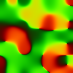
We can conjure tensor fields from the Aether and pretend that whatever dynamics they encode pertain to some noise image. The noise image is unrelated to the tensor field and that is atypical. Commonly, a tensor field relates to a corresponding image through the action of some analytic G'MIC command like -structuretensors or -diffusiontensors, but in this application we're pursuing Art. Perhaps, more precisely, we are using noise to visualize a tensor field. The results can be quite pretty.In any case, we will first conjure from the Aether the eigenvalue and eigenvector components. We will conjure up four gray scale images: Eigen One, Eigen Two, Cosine, and Sine. This terminology comes from Do Your Own Diffusion Tensor Fields which (we think) might be worth your while to read.
| Eigen One | Eigen Two |
 |  |
gmic \
-repeat 2 \
5,5,1,1,'2*u-1' \
-resize2dx. 300,5 \
-done \
-normalize[-2] 0,0.75 \
-normalize[-1] 0.25,1 \
-repeat 2 \
5,5,1,1,'2*u-1' \
-resize2dx. 300,5 \
-done \
-normalize[-2] 0,0.75 \
-normalize[-1] 0.25,1 \
| 1. | We hereby declare that these two images are, respectively, EigenOne and EigenTwo, datasets describing pixel-level intensity dynamics for some yet-to-be conjured PrettyPicture. Normally one computes such from pre-existing pretty pictures, but we are in contrary moods and prefer putting carts before horses. Or, perhaps, computing the intensity dynamics of an image before the image even exists. |
| The datasets started out as 5 × 5 noise fields; note the 2*u-1 generator attached to the image specification. We resize with a cubic interpolator and then normalize each to a pair of ranges: EigenOne to [0.00, … 0.25] and EigenTwo to the range [0.75, … 1.00]. | |
| Why for??? At the end of the day, when smooth is at the helm, it uses EigenOne and EigenTwo as the axial lengths of elliptical "blur brushes", one blur brush for each target image pixel. The differing ranges means the elliptical blur brushes will be, on the whole, longer in one direction than the other - it will blur more in one direction than the other. |
Elliptical Brush
| Eigen One | Eigen Two | Cosine + Sine |
 |  |  |
-input 7,7,1,2,2*u-1 \
-resize. [-2],[-2],[-1],[-1],5 \
-orientation. \
-resize. [-2],[-2],[-1],[-1],5 \
-orientation. \
| 2. | Next we conjure Cosine and Sine from a similarly randomized field, scaling it through resize 's cubic interpolator and harnessing orientation to normalize this image. This step produces unit length, two dimensional rotation vectors. At the end of the day, smooth consults this Cosine and Sine data set to determine, pixel by pixel, how to orient the blur brush. This two channel image essetially sets the orientation of the blur brushes, while Eigen One sets the length, and Eigen Two sets the width of the blur brushes. These are the operating components of a tensor field: pixel-by-pixel instructions to size and rotate a blur brush for each.. |
| Eigens | Cosign + Sine | Tensors | Pretty Noise |
 |  |  |  |
-append[^-1] c \
-eigen2tensor[-2,-1] \
-input 100%,100%,1,3 \
-noise[-1] 8,2 \
-dilate_circ 3 \
-rgb2hsl[-1] \
-split[-1] c \
-mul[-3] 0.5 \
-add[-3] 135.0 \
-append[-3,-2,-1] c \
-hsl2rgb[-1] \
-normalize[-1] 0,255 \
-eigen2tensor[-2,-1] \
-input 100%,100%,1,3 \
-noise[-1] 8,2 \
-dilate_circ 3 \
-rgb2hsl[-1] \
-split[-1] c \
-mul[-3] 0.5 \
-add[-3] 135.0 \
-append[-3,-2,-1] c \
-hsl2rgb[-1] \
-normalize[-1] 0,255 \
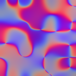
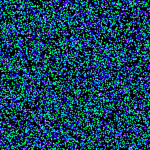
| 3. | We pack Eigen One and Eigen Two into a two-channel image (Eigens) and invoke eigen2tensor to generate a tensor field. This purple/red/blue/grey kind of swirly image is what we are harnessing as a smoothing geometry, to wit: per-pixel instructions to build a blur brush centered over each pixel in the target image. Alas! What we don't have is the target image. For now, we'll generate some pretty noise and use that as a target image. |
| Pretty Noise Recipe: (a) Make salt-and-pepper noise in three RGB channels. (b) Convert same to HSL and (c) split out the channels for color work. (d) The color work consists of (-i-) scaling the color space to one half and (-ii-) adding a color offset of 135°. This compresses the color range to around a cyan, blue, magenta colorwheel wedge. (e) We could mess with saturation but we won't. (f) We could also mess with luminance but we won't. (g) We append the three separated channels back into one image and (h) bring that image back into RGB color space. (i) Normalizing the image to the range [0...255] corrects any range issues our color surgery may have created. That's the gist of the ten noise maker G'MIC commands following eigen2tensor. | |
| Pretty Noise is the prototype of our ersatz Pretty Picture. Being a uniform random pattern of points, Pretty Noise is especially sensitive to the aggregate behavior of the smoothing geometry encoded in Tensors. We can imagine this field as being comprised of small ellipses, our blur brushes, at various sizes, eccentricities and orientations, with each ellipse centered on a pixel. Some will blur isotropically – rather the same way in all directions. Other ellipses, the more eccentric ones, will be distinctly anisotropic in character and smooth only in particular directions. The command display_tensors visualizes the ellipses in a tensor field. See the tutorial on structuretensors for a working example. |
| Tensors | Pretty Noise | Pretty Picture |
 |  |  |
-repeat 3 \
-smooth[-1] [-2],100 \
-done \
-rm[0] \
-normalize[-1] 0,255 \
-apply_gamma[-1] 3.5 \
-output[-1] ppict.png
-smooth[-1] [-2],100 \
-done \
-rm[0] \
-normalize[-1] 0,255 \
-apply_gamma[-1] 3.5 \
-output[-1] ppict.png
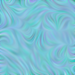
| 4. | Our PrettyPicture after three passes using smooth. |
| With practice, one can read the behavior of the tensor field from the faux color display. Saturated blue and red regions both correspond to very elliptic tensors; blue has a very strong vertical bias, red a horizontal one. These colors engender very anisotropic blurring. The noise pattern elongates into hairlike patterns. | |
| Other areas exhibit less strongly oriented blurring and correspond to areas of less saturated hue. | |
| Finally, gray areas have little or no directional bias whatsoever. These areas behave very much like conventional isotropic blurring kernels. |

Command reference
$ gmic -h eigen2tensor
eigen2tensor:
Recompose selected pairs of eigenvalues/eigenvectors as 2x2 or 3x3 tensor fields.
Tutorial: https://gmic.eu/tutorial/eigen2tensor
eigen2tensor:
Recompose selected pairs of eigenvalues/eigenvectors as 2x2 or 3x3 tensor fields.
Tutorial: https://gmic.eu/tutorial/eigen2tensor


 Home
Home Download
 News
News Mastodon
 Bluesky
 X
X Summary - 17 Years
 Summary - 16 Years
 Summary - 15 Years
 Summary - 13 Years
 Summary - 11 Years
 Summary - 10 Years
 Resources
 Technical Reference
 Scripting Tutorial
 Video Tutorials
 Wiki Pages
 Image Gallery
 Color Presets
 Using libgmic
 G'MIC Online
 Community
 Discussion Forum (Pixls.us)
 GimpChat
 IRC
IRC Report Issue