rbf
| Given a sparse set of keypoints, rbf reconstructs an approximation from a weighted set of radial basis functions, (RBFs), each taking an observed keypoint as a parameter. -rbf finds weights from a least squares fitting; the solution interpolates keypoints and estimates fits for locations in between these. -rbf can reconstruct approximations from about 1,000 keypoints taken from 1000 × 1000 images, the results dependent on both the sampling pattern and the particular kind of RBF used. Among other uses, G'MIC employs -rbf to compress color look up tables (CLUTs), where a sparse sampling of the original provides a compact representation. The behavior of the reconstructed CLUT differs little from the original. Another congenial setting for RBFs may be found in simulated neural networks. Here, RBF meshes integrate stimuli and respond to particular patterns by "firing" an output pulse. |
Given two numerals, 3 and 7, one could guess at an in-between value of 5. On what basis does that guess sit? Well — none, really. It stems from some heuristic that, knowing nothing else about extremes then in-betweens are as likely as anything else. Thus the art of reconstruction: given (a very few) hints, interpolate the whole as so many averages. The technique here entails basis functions, a kind of simple-to-compute template function that scales, slides around and from a very few keypoints estimates what goes on in between them.
Radial basis functions (RBFs) are one such type of basis function, so-called because these functions,
 take only a radius r and return a "relative contribution". That reflects what a known keypoint contributes to an approximation at a radial distance r. This radius is itself a proxy for a difference that we take between two locations: the place where we are making our assessment, x, and the place where the sample has been "observed" c. A suitably weighted set of RBFs
  can approximate an entire image through a small set of keypoints so long as some loss is acceptable.
rbf, given a set of keypoints, returns a range image computed from the keypoints, as processed by the set of weighted RBF's. The keypoints may be drawn from one, two or three dimensional spaces and the range has a like number. We can take an inconveniently large data set — a color look-up table (CLUT) — and save selected keypoints, these consuming just a fraction of the storage of the original. Later on, we could reconstruct the CLUT from the keypoints and obtain something that almost matches the original. Is it the original? No. Does it work like the original? It could work in a pretty fair dinkum sort of way, with an adroitness to the sampling and an apt choice of RBFs; that is a deep topic upon the edge of which we teeter. For safety's sake, let's assume a sampling fair and RBFs robust. This brings us to particulars:
| 1. | We obtain keypoints — "spot-checks" — for an otherwise unknown image. |
| 2. | -rbf plots approximations into one, two or three dimensional images: the range. |
| 3. | Arguments to -rbf quantify the range for ·: x, y or z. |
| a. | d· arguments specify range dimensions and lengths; these are required. |
| b. | ·0 arguments specify origin offsets; their absences imply zero offsets. |
| c. | ·1 arguments specifies the dimensional lengths of the sample space; their absences imply that the sample and range spaces have equally sized dimensions and that scaling is 1:1. |
| d. | A final, optional string is taken to be a math expression and defines a custom RBF. Its absence implies the default RBF, the thin plate spline, described further on. |
| 4. | The images referenced in -rbf's selection decorator are one dimensional vectors encoding keypoints. Each pixel encodes keypoints in spatial coordinate-sample value order; two coordinates and three values codify the position and color of an RGB sample, for example. Each datum occupies separate channels. -rbf separates coordinate from value channels by determining the number of dimensions of the output range. This arises from particular argument signatures: |
| a. | one, three or four arguments: one dimensional ranges. Signatures may consist of 1 argument: Only the length of the range: dx. They may consist of 3 arguments: Range length with origin offset x0 and the sample space dimensional length x1; dx:x1 sets scaling from range to sample space. They may consist of 4 arguments: Those before plus a custom RBF, written as a math expression. |
| b. | two, six and seven arguments: two dimensional ranges. Signatures may consist of 2 arguments: Only the length of the range in dx and dy. They may consist of 6 arguments: Range length in dx and dy, origin offsets, x0 and y0 and the sample space dimensional lengths x1 and y1. They may consist of 7 arguments: Those before plus a custom RBF, a math expression. |
| c. | nine and ten arguments: three dimensional ranges. Signatures may consist of 9 arguments: The length of the range in dx, dy and dz, origin offsets x0, y0 and z0 and the sample space dimensional lengths x1, y1 and z1. They may consist of 10 arguments: Those before plus a custom RBF, a math expression. |
| 5. | "Decompressing" a sparse set of keypoints into an approximation range entail finding weights for each of the RBF's, so that associated keypoints may be appropriately scaled. This is taken as a least squares problem; G'MIC composes a design matrix D by taking the absolute values of pairwise differences among the given keypoints and evaluating these with the chosen RBF. The design matrix which arises from this exercise is symmetric, the lower diagonal mirroring the upper. A linear least squares approach solves for the weights of the RBFs: |


Various Radial Basis Functions recreate 1-D estimated functions from six sample points.
| 1. | Blue dots | Six sample points | |
| 2. | Purple |  | Lerps the keypoints. |
| 3. | Olive |  | Unscaled Gaussians. |
| 4. | Light Green |  | Scaled Gaussians. The frontpiece animation illustrates a progression of ε from 1.0 → 0.01. |
| 5. | Orange |  | Thin plate spline, the default radial basis function. Its behavior between keypoints is reminiscent of spring steel strips. |
Examples
Reconstruct an image twice from 16 random samples, using the inverse multiquadric RBF, then the thin plate spline.| 1. | Inverse Multiquadric Stars | Thin Plate Spline Stars |
 |  | |
 |  |
starfield:
-srand 1234 # Choose the start point of
# a random sampling
-16,1,1,5,'u([256,256,255,255,255])' # Get sixteen random samples
# as a 1-D × 5 channel vector
+rbf. 256,256 # Reconstruct from thin plate
# spline RBF (default)
-rbf.. 256,256,0,0,255,255,'sqrt(1/(1+0.01*r^2))' # Reconstruct
# from inverse multiquadric
-normalize 0,255 # Normalize to 2^8
§§§
| 2. | Colorful Cupid | Colorful Cupid Sampled | Thin Plate Reconstruction | Scaled Gaussian Reconstruction |
 | 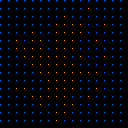 |  | 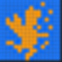 |
reconstruct_cupid:
-shape_cupid 256 # Make a colorful cupid
-to_rgb. # from the [0,1] binary
-fill. lerp([0,1,0],[1,0,1],i) # Lerp between green and
# magenta
-adjust_colors. 0,0,0,53,100 # Twist it toward orangish
# and bluish
-normalize. 0,255 # Normalize to 2^8
-name. cupid # Call image 'cupid'
-input 100%,100%,1,1 # Sample cupid at every
# 8th pixel left-to-right,
-fill. x%8==0&&y%8==0 # top-to-bottom
-name. keypoints # Keypoints for reconstruction
slen={is} # Image sum = sample count because
# template has zero or one booleans
-mul[-2,-1] # Fetch samples: image × template
-input $slen,1,1,5 # Package samples into a 1-D,
-eval[cupid] ">begin(p=0); # 5-channel vector
norm(I#-2)>0?
I[#-1,p++]=[x,y,I#-2]
"
-name. samplevector # Keypoint vector for rbf
+rbf[samplevector] 256,256 # Thin plate spline
-rbf[samplevector] 256,256,0,0,255,255,exp(-0.035*r^2)
-normalize 0,255 # Scaled Gaussian
§§§
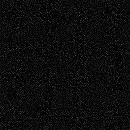
| 3. | Orientation | Markers | Plotted Ellipses |
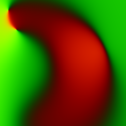 |  | 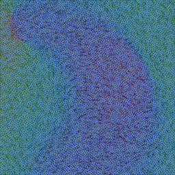 |
orientedellipses:
-srand 5823619
# Make a field of orientation angles through RBF interpolation
6,1,1,4,{[u(2047),u(2047),u(2047),u(2047),u(2047),u(2047),\
u(2047),u(2047),u(2047),u(2047),u(2047),u(2047),\
u(-1,1),u(-1,1),u(-1,1),u(-1,1),u(-1,1),u(-1,1),\
u(-1,1),u(-1,1),u(-1,1),u(-1,1),u(-1,1),u(-1,1)]}
-rbf. 2048,2048
-orientation
-name. orient
# Markers to place ellipses
-input 100%,100%,1,1
-noise_poissondisk. 20
-name. markers
# Plotting field. Give it a shadow
# of the orientation field
-input 100%,100%,1,3,'[90,30,40]'
-name. plottingfield
-fill[plottingfield]
">begin(wv=vector3(1/sqrt(3)));
rot(wv,atan2(i(#-3,x,y,0,1),i(#-3,x,y,0,0)))*I"
# Plot the ellipses themselves, aligned
# with the orientation field.
-fill[plottingfield]
">if(
i#-2>0,
ellipse(#-1,x,y,12,18,atan2(i(#-3,x,y,0,1),i(#-3,x,y,0,0)),0.5,[63,127,255]);
ellipse(#-1,x,y,-12,-18,atan2(i(#-3,x,y,0,1),i(#-3,x,y,0,0)),1,0xffffffff,[255,255,0]);
I,I
)
"
-keep.
-rs. 50%,,5
-normalize. 0,255
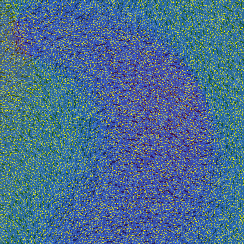
oriented ellipses
Command Reference
$ gmic -h rbf
rbf:
dx,_x0,_x1,_phi(r) |
dx,dy,_x0,_y0,_x1,_y1,_phi(r) |
dx,dy,dz,x0,y0,z0,x1,y1,z1,phi(r)
Reconstruct 1D/2D or 3D image from selected sets of keypoints, by RBF-interpolation.
A set of keypoints is represented by a vector-valued image, where each pixel represents a single keypoint.
Vector components of a keypoint have the following meaning:
- For 1D reconstruction: [ x_k, f1(x_k),...fN(x_k) ].
- For 2D reconstruction: [ x_k,y_k, f1(x_k,y_k),...,fN(x_k,y_k) ].
- For 3D reconstruction: [ x_k,y_k,z_k, f1(x_k,y_k,z_k),...,fN(x_k,y_k,z_k) ].
Values 'x_k','y_k' and 'z_k' are the spatial coordinates of keypoint 'k'.
Values 'f1(),..,fN()' are the 'N' components of the vector value of keypoint 'k'.
The command reconstructs an image with specified size 'dx'x'dy'x'dz', with 'N' channels.
Default values: 'x0=y0=z0=0', 'x1=dx-1', 'y1=dy-1', 'z1=dz-1', 'phi(r)=r*log(1+r)'.
Example:
[#1] sample colorful,400 100%,100% noise_poissondisk. 10 1,{is},1,5 eval[-2] "begin(p=0);i?(I[#-1,p++]=[x,y,I(#0)])" to_rgb[1] mul[0,1] dilate_circ[0] 5 +rbf[-1] {0,[w,h]} c[-1]
0,255
[#2] 32,1,1,5,u([400,400,255,255,255]) rbf 400,400 c 0,255
Notes
| dx,dy,dz | Sets the output range, in pixels. dx, in isolation, implies a one dimensional output range. dx,dy implies a two dimensional output range. dx,dy,dz implis a three dimensional output range. Must be specified (no defaults). |
| -x0,y0,z0 | Origin: Sets what output coordinate, ·0, corresponds to input origin 0. Provide as many origin coordinates ·0 as there are output ranges d·. Defaults to 0. |
| -x1,y1,z1 | Scaling: d·:·1. Sets what input range, ·1, corresponds to output range d· Provide as many input ranges ·1 as there are output ranges d·. Set ·1 = d· for 1:1 scaling from input to output. Set ·1 = 2*d· for 50% downscaling from input to output. Defaults to d· – 1. |
| phi(r) (math expression) | Set the radial basis function. The default, r^2*log(1e-5+r) provides the thin plate spline. The math expression recognizes the symbol r (radius) as representing the Euclidean distance xy — c between image points xy and keypoints c. During evaluation of the basis function, G'MIC's math parser substitutes for r, wherever it may appear in the expression, the Euclidean distance. Other expressions may be provided, over-riding the default. Ensure that the math expression is written in terms of just one variable, r. |


 Home
Home Download
 News
News Mastodon
 Bluesky
 X
X Summary - 17 Years
 Summary - 16 Years
 Summary - 15 Years
 Summary - 13 Years
 Summary - 11 Years
 Summary - 10 Years
 Resources
 Technical Reference
 Scripting Tutorial
 Video Tutorials
 Wiki Pages
 Image Gallery
 Color Presets
 Using libgmic
 G'MIC Online
 Community
 Discussion Forum (Pixls.us)
 GimpChat
 IRC
IRC Report Issue