 Home
Home Download
 News
News Mastodon
 Bluesky
 X
X Summary - 17 Years
 Summary - 16 Years
 Summary - 15 Years
 Summary - 13 Years
 Summary - 11 Years
 Summary - 10 Years
 Resources
 Technical Reference
 Scripting Tutorial
 Video Tutorials
 Wiki Pages
 Image Gallery
 Color Presets
 Using libgmic
 G'MIC Online
 Community
 Discussion Forum (Pixls.us)
 GimpChat
 IRC
IRC Report Issue
orientation

usphere.png
The point on the unit sphere is pure hue. The volume in the sphere contain shaded hues. Tints live outside.

In the resulting image, pixel RGB components plot points on a unit sphere centered on the origin of the RGB color space. A line passing through the origin and the corresponding plot consists of points with the same hue, differing only in luminosity. Informally, the plot itself represents the "pure" hue, with colors tending toward the origin being shades of, and those tending away from the origin being tints of the pure hue.
An image transformed by orientation is an apt dataset for a number of color selection and identification algorithms. How dark or light a pixel may be has been put to one side and only chromatic data remains.
The RGB Color Space

ccube.png
The point at (236,193,95) is in a kind of a yellow brown part of the color cube
We can regard a color's red, green and blue components as a position vector in some three dimensional RGB color space (see mix_rgb), with the "tail" rooted at the origin and the "head" plotting the color itself.
Vectors express both direction and length. The RGB color space which color vectors comprise has a Euclidean metric: a means to find "distance" between points comprising the space. We find the length of color vectors by taking the square root of the sum of squared color components: see Pythagorean formula.
There are circumstances when we'd like to consider the length, or magnitude, of a color vector quite apart from the direction in which it points. In G'MIC, norm extracts that information, producing a grayscale counterpart of a color image where the intensity of pixels reflect the RGB color space length of their counterparts.
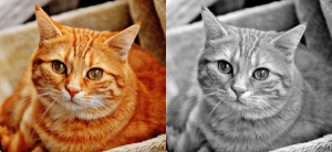
normed_cat.png
In contrast, orientation extracts the RGB space orientation of a color vector quite apart from its length. This entails scaling each color component of a pixel by the length of the vector which those components define, producing a triplet of unitless numbers, also composing a vector, but one of unit length.
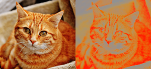
oriented_cat.png
These triplets describe the orientation of colors in RGB space. One can imagine an open-ended line starting at the the origin and passing through the plot on the unit sphere. The direction in which this line points is a shared characteristic of all the colors on that line. They share a common orientation – a common hue – but differ in their luminance. See usphere.png.
Unsurprisingly, orientation produces a flat version of its original, generally unappealing, with the shadows and highlights of the original no longer present; both transit to a midlevel gray. The more saturated colors of the original generally become the prominent features of the processed image, which may or may not be appealing. Since the pixels in the resulting image are either zero or one, they are not directly suitable in paint programs and need to be normalized before use with such tools. See Images as Datasets.
orientation almost always is a means to an end and rarely an end in itself. While it might not make pretty pictures, the catalog of unit vectors it creates underlies color search and manipulation schemes.
Examples
![sp monkey,150 +norm. to_rgb. +orientation.. normalize[^0] 0,{2^8-1}](img/sp_monkey_150_norm_to_rgb_orientation_normalize_0_0_2_8_1_.png)
bluemonkey.png
The norm and orientation of a blue monkey
gmic \
-sample monkey,300 \
+norm[-1] \
+orientation[-2]
-sample monkey,300 \
+norm[-1] \
+orientation[-2]
Euler angles provide the means to do rigid body rotations in the RGB color space. We may twist the "R", "G", or "B" axes with the aim of doing color adjustments. In the following example, we do just that: alter the orientation of the color vectors. In the course of doing that, we shift the hues of the image. As an added twist, we will use the norm part of the decomposition to restrict the adjustment mainly to the shadows, somewhat in the mid tones, but hardly affect the orientation of the highlights at all.
| Original | Color Vectors | Vector Lengths | Factors |
 |  |  |  |
gmic \
-sample monkey,150 \
+orientation[-1] \
+norm[-2] \
+normalize. 0,1 \
-oneminus. \
-sample monkey,150 \
+orientation[-1] \
+norm[-2] \
+normalize. 0,1 \
-oneminus. \
| Original | "G" rotation | Vector Lengths | Factors |
|  | | |
fill... "ang=-40.0; \
cz=cos(pi*ang*i#-1/180); \
sz=sin(pi*ang*i#-1/180); \
[[cz,0.0,sz],[0.0,1.0,0.0],[-sz,0.0,cz]]*I#-3" \
cz=cos(pi*ang*i#-1/180); \
sz=sin(pi*ang*i#-1/180); \
[[cz,0.0,sz],[0.0,1.0,0.0],[-sz,0.0,cz]]*I#-3" \
What is going on here? Broadly, we are using a G'MIC math expression to apply an Euler angle to twist an axis - here the "G" axis - that connects green and its complement magenta. It is the "middle" axis of the RGB color space and could be thought of as the "Y" axis. We harness fill to apply the math expression to every pixel in the target image. That is, fill "marches over" the target image first by columns, then by rows, until it has visited each pixel in the target image. At each visit, it sets the value of a number of standard variables pertaining to the pixel, then performs the computation of the math expression. We'll discuss some of those standard variables in the breakdown of this expression, which follows.
And what is the target image? That is what the three "..." dots do following the fill command. They are a convenient alias for the [-3] image selection decorator. Counting from the end of the image list, the three dots take us past the multiplication factors (.), past the normed vector lengths (..) and selects the Color vectors (...), the target image, which the math expression operates on.
The math expression itself may seem imposing, but lets break it down.
| 1. | The first line is a convenient "control line". We define a variable ang and set it to -40.0°. That is, our first Euler operation is to twist the "G" axis by at most -40.0°, a clockwise twist. Absent the minus sign, it would be a counterclockwise twist. We say "at most" because we intend to regulate the actual rotation by the scaling factors contained in the last image on the list. Recall that these multiplication factors are the relative inverse of the norms; they are one or nearly so for dark shadow pixels, but zero or nearly so for the highlights. We twist the axis the most for shadow pixels and least for the highlights. |
| 2. | The second line conputes the cosine of the actual twisting angle. How we find the actual twisting angle takes place within the parentheses of the cos() function. Most of it is Old School conversion from degrees to radians, which the cos() function requires: pi*ang/180 where pi is a built-in variable representing 3.1415926.... The interesting variable here is i#-1. Read this as shorthand for the intensity (i) of the pixel in the last image on the list (#-1) - aka, the multiplicitive factor to regulate the actual rotation angle. This "Hashtag-number" notation is the math expression analog of the image selector [-1] and it shares the same numbering convention: negative sign selectors count from the end of the list; positive selectors count from the beginning of the list. See Command Decorations. i is another built-in variable representing the intensity of the current pixel the math expression is centered on. Taken together, then, this expression computes the cosine of a rotation angle that is at most -40.0°, but can be "dialed back", on a pixel-by-pixel basis, by the multiplication factors taken from the last image on the list. |
| 3. | The third line has been composed nearly identically to the second, and what was written about that line applies to this one as well. The only difference is that it computes the sine of the actual rotation angle. How these two factors, sz and cz, give rise to a rotation takes place in the next line, where we rotate a Color vector by its corresponding rotator, one of the standard Euler Rotation Matrices; sz and cz are incorporated into this rotator. |
| 4. | The fourth line realizes a matrix multiplication between the rotator and the color vector in the target image. Rearrange the notation in the square brackets, and see that they form a 3X3 block of numbers: a matrix. Without going into too much detail, matrices have the property of moving vectors from one to another place: Broadly, matrices can translate, rotate, scale - generally transform - objects like vectors into new positions, orientations and sizes. |
| In our application, we want to rotate the color vectors so that they occupy, or point to, more blue-like regions on the surface of the color sphere (recall usphere.png at the start of this article). The Euler rotation matrices are so patterned to produce only rotations about specific axes. They don't scale. They don't translate. In this case, we plug in sz and cz into the appropriate places for "G" axis rotation. For reference, here are the "R" "G" and "B" rotators: |
![R_{red}(\theta) &= \begin{bmatrix} 1 & 0 & 0 \\ 0 & \cos \theta & -\sin \theta \\[3pt] 0 & \sin \theta & \cos \theta \\[3pt] \end{bmatrix} \\[6pt] R_{green}(\theta) &= \begin{bmatrix} \cos \theta & 0 & \sin \theta \\[3pt] 0 & 1 & 0 \\[3pt] -\sin \theta & 0 & \cos \theta \\ \end{bmatrix} \\[6pt] R_{blue}(\theta) &= \begin{bmatrix} \cos \theta & -\sin \theta & 0 \\[3pt] \sin \theta & \cos \theta & 0\\[3pt] 0 & 0 & 1\\ \end{bmatrix}](img/R_red_theta_begin_bmatrix_1_0_0_0_cos_theta_sin_theta_3pt_0_sin_theta_cos_theta_3pt_end_bmatrix_6pt_R_green_theta_begin_bmatrix_cos_theta_0_sin_theta_3pt_0_1_0_3pt_sin_theta_0_cos_theta_end_bmatri.png)
You probably can see that these are none other than the rotators for X ("R red"), Y ("R green") and Z ("R blue"), lightly relabeled.
We employ these rotators to turn color vectors. The notation I#-3 is the vector (or pixel) form of what we have already encountered with i. The hashtag-number form selects a vector in the Color vector image. We could have omitted this decoration - the target image already is the Color vector image - but sometimes extra redundancy reminds us of the role a variable is playing.
When the math processor encounters this fourth line and rotates the color vector it has finished. What happens next? By math processor conventions, the last value computed in the expression becomes the results that are passed back to the target image. Here, I#-3 has its component RGB values changed in such a way that the overall color vector has now been rotated on the "G" axis by as much as -40.0°, but probably less, given the "dialing back" value of i#-1. That rotated vector becomes the new pixel. Now fill continues on, "filling" the target image with a computed stream of pixels.
If the math expression here still seems incomprehensible, see the fill command itself, where a gentler introduction to math expressions may be found.
| Original | "G+R" rotation | Vector Lengths | Factors |
|  | | |
-fill... "ang=20.0; \
cz=cos(pi*ang*i#-1/180); \
sz=sin(pi*ang*i#-1/180); \
[[1.0,0.0,0.0],[0.0,cz,-sz],[0.0,sz,cz]]*I#-3" \
cz=cos(pi*ang*i#-1/180); \
sz=sin(pi*ang*i#-1/180); \
[[1.0,0.0,0.0],[0.0,cz,-sz],[0.0,sz,cz]]*I#-3" \
And then we twist again -- but, wait! There are differences here. For one, the angle has changed. We are rotating at most 20.0° in the counterclockwise (positive) direction - and the rotator has changed. cz and sz are arranged in a different pattern. This pattern is for rotations along the "R" axis, running from red to its complement cyan. Apart from that, the mechanics of this fill command is very much the same as the previous one.
![v - img/m3.cimg rm. mul[-2,-1] normalize 0,{2^8-1}](img/v_img_m3_cimg_rm_mul_2_1_normalize_0_2_8_1_.png)
-rm. \
-mul[-2,-1] \
-normalize. 0,'{2^8-1}' \
-output. bluer_monkey.png
-mul[-2,-1] \
-normalize. 0,'{2^8-1}' \
-output. bluer_monkey.png
Postscript
Some of you may react with a "Big Deal! All this work for what can be simply done with adjust_colors!"Look again. Try as you might, you will not get this particular effect with adjust_colors alone. You might hit the fur, but the eyes go green. Get the eyes right but the fur goesoff to violet. You'll start pulling in masks to single out regions - and it will no longer something that could simply be done with adjust_colors.
We turned to this particular math expression because it offers more degrees of freedom - individual control of the color axes - than what a single rotation along a color wheel can afford. Nor does a tool like adjust_colors allow for per-pixel value adjustments, such as what we did with the multiplication factor image. adjust_colors is good. It achieves a great deal with an economy of form. But some problems require operations at a finer scale. That's when having a grasp of G'MIC math expressions becomes very significant because they operate at the pixel level.
And there are those on the other end of the spectrum, experienced scripting people, looking gimlet-eyed at me and muttering "Ugh! All this inefficient code!" Certainly. The two fills can easily be combined into one, with the two rotation matrices composed together. We've already noted that I#-3 is redundant in that context: It is in the target image already and I suffices. But when one is exploring, I find it best to keep the code "unrolled" as much as possible so that the component pieces are easily grasped. Once grasped, then "roll it up" into production code. More efficient, yes, and probably harder to debug.
Command reference
$ gmic -h orientation
orientation:
Compute the pointwise orientation of vector-valued pixels in selected images.
Example:
[#1] image.jpg +orientation +norm[-2] negate[-1] mul[-2] [-1] reverse[-2,-1]
Tutorial: https://gmic.eu/tutorial/orientation
orientation:
Compute the pointwise orientation of vector-valued pixels in selected images.
Example:
[#1] image.jpg +orientation +norm[-2] negate[-1] mul[-2] [-1] reverse[-2,-1]
Tutorial: https://gmic.eu/tutorial/orientation