 Home
Home Download
 News
News Mastodon
 Bluesky
 X
X Summary - 17 Years
 Summary - 16 Years
 Summary - 15 Years
 Summary - 13 Years
 Summary - 11 Years
 Summary - 10 Years
 Resources
 Technical Reference
 Scripting Tutorial
 Video Tutorials
 Wiki Pages
 Image Gallery
 Color Presets
 Using libgmic
 G'MIC Online
 Community
 Discussion Forum (Pixls.us)
 GimpChat
 IRC
IRC Report Issue
map
A mapping from gray to color
Map assigns palettes of reference colors to index maps. The index map is a single channel gray scale. The numeric values of its pixels are taken to be indices which select colors from a given palette of reference colors.
Informally, map is the "paint-by-numbers" command. The palette corresponds to a box of enumerated paints; these can't be mixed nor used from somewhere else. The index map corresponds to the card printed with various enumerated regions. The painter corresponds to the map command; he or she looks at the card and paints regions the color corresponding to the number printed in the region.
In a restricted sense, map is the inverse operator of index. When one sets that command's map_palette parameter False, index produces a single channel gray scale image, the index map. its pixels contain indices that assign reference colors from the palette to the pixels. The map command produces a new image by following all of the assignments indicated in the index map.
In a less restricted sense, one may regard any gray scale image as an index map; such need not be produced by index. Taking this liberty, then map becomes a tool to convert gray scales into "false color" images.
One practical aim of this idea is to make lucid features that are not particularly clear in some gray scale representation of a phenomenon. One makes a correspondence between gray levels and color (i. e., constructs a palette of reference colors) and then makes astute color assignments for those very nearly identical grays that are difficult to distinguish.
Example
Root polishing by Newton's method entails using a succession of trial values starting from initial guesses. These trial guesses take the form of complex numbers, x + iy. Some guesses converge very rapidly toward the roots of a given polynomial; others do not converge until thousands of iterations have taken place and some guesses never converge. This difference in behavior can be harnessed to visualize the basins of attraction for polynomial roots. See newton_fractal for generating images of these basins of attraction and their mathematical significance.It turns out that the basin of attraction for a particular root is a really quite fantastic, fractal shape if the degree of the associated polynomial is two or higher. Sometimes rendering problems occur, however. Significant detail may be masked because they have been rendered in very similar shades. This is the kind of conundrum that map can fix.

basin_index_map.png
Basin of attraction
A basin of attraction for one of the roots of some polynomial. Very dark gray corresponds to parts of the basin which take a very large number of iterations before converging on a root, but absolute black corresponds to other basins of attraction.
`Tis not a very distinct distinction.

map_palette_31y.png
256 step palette. Only the top row needed, but adding thirty more duplicate rows increases the height and it is easier to see the palette.
![images/basin_index_map.png images/map_palette_31y.png map.. [-1] rm.](img/images_basin_index_map_png_images_map_palette_31y_png_map_1_rm_.png)
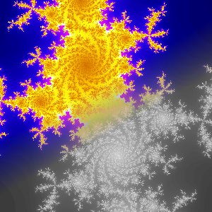
basin.png
gmic \
input basin_index_map.png \
input map_palette_31y.png \
map[-2] [-1],0 \
remove[-1] \
output[-1] basin.png
input basin_index_map.png \
input map_palette_31y.png \
map[-2] [-1],0 \
remove[-1] \
output[-1] basin.png
The key takeaway is that map made clear a pattern that is obscure and could otherwise escape our attention. But, with a new phenomenon made lucid through map, we now have an interesting line of investigation in our studies of complex math.
Command reference
$ gmic -h map
map (+):
[palette],_boundary_conditions |
palette_name,_boundary_conditions
Map specified vector-valued palette to selected indexed images.
Each output image has 'M*N' channels, where 'M' and 'N' are the numbers of channels of, respectively, the corresponding input image and the 'palette' image.
'palette_name' can be { default | hsv | lines | hot | cool | jet | flag | cube | rainbow | algae | amp | balance | curl | deep | delta | dense | diff | gray |
haline | ice | matter | oxy | phase | rain | solar | speed | tarn | tempo | thermal | topo | turbid | aurora | hocuspocus | srb2 | uzebox }
'boundary_conditions' can be { 0:Dirichlet | 1:Neumann | 2:Periodic | 3:Mirror }.
Default value: 'boundary_conditions=0'.
Example:
[#1] image.jpg +luminance map[-1] 3
[#2] image.jpg +rgb2ycbcr split[-1] c (0,255,0) resize[-1] 256,1,1,1,3 map[-4] [-1] remove[-1] append[-3--1] c ycbcr2rgb[-1]
Tutorial: https://gmic.eu/tutorial/map
When this parameter is an image selection (a numeric index in square brackets), the selected image is taken to be a single row, multicolumn set of reference colors, regardless of the image dimensions. The command indexes the pixels in the reference image from left-to-right, top-to-bottom, taking each pixel to be a reference color. While the image may be any size, it is rarely practical to have more than a few hundred reference colors, and a few dozen are usually ample. The image is almost always quite small.
When this parameter is a name, it is taken to be a reference to a number of built-in color lookup tables.
To preview these named palettes, consider:
gmic 256,256,1,1,'x' +map < *palette name* >

The hocuspocus palette visualized
This places a gray ramp on the left, in this example having 256 steps, and the palette on the right - the colors to which specific gray levels on the left translate.
2. boundary: (0) Sets policy when indices in the map reference colors outside the range of the palette:
a. dirichlet: (1) Assume the color beyond the reference palette is black.
b. neumann: Assume the color beyond reference palette is the same as that of the largest index value.
c. cyclic: (2) Replace the out-of-bounds index, k with r = k modulo p, where p is the length of the pallete. That is, indices exceeding the length of the palette “wrap around” to the beginning of the palette. The color appearing in the output corresponds to r.
d. mirror: (3) Past the image boundary, the palette entries are used in reverse.