A Full-Featured Open-Source Framework for Image Processing

do…while (+)

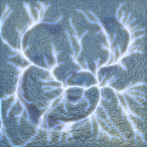Caution: Electrified 1911 Goudy Bookletter Ampersand. Please do not stand in any water puddles or other conductive liquids while following this tutorial. Thank you.

The -do <loop scope> -while commands form a syntactical unit that repeatly executes in-scope commands until -while's argument resolves to False. Execution continues with the commands after -while. -do…-while expresses a "perform, then test" pattern. With the conditional test at the bottom of the loop, the in-scope commands execute once even if -while's mathematical expression is initially False. For a "test, then perform" pattern, consider for … done. The <loop scope> need not be populated and is a placeholder when empty. Prior to 2.6, -while would test file system references. This is no longer supported. Use the file system mathematical expressions isfile() or isdir() instead.

Examples

dowright:    -do       -echo "You'll never take              me alive, Dudley              Do-right!!!"    -while bool(1)

Snidely Whiplash won't shut up until Ctrl-C intervenes. Commands within <loop scope> execute forever if -while's argument remains stuck on True. Consider a testable -while condition or build an 'escape hatch' within <loop scope> with the break command, often in the scope of an if … fi block. Similarly, continue terminates the current iteration and forces an immediate re-evaluation of -while's conditional argument.

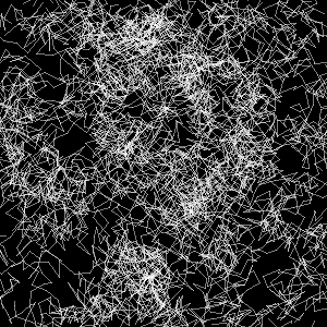5000 steps of Brownian motion

Usually, the commands constituting the body of the <loop scope> have some direct or indirect effect on the mathematical expression given as an argument to -while. -wanderaround, listed below, draws specific counts of random-length, randomly oriented segments, end-to-end, on the currently selected image. It checks for boundary overshoot, wrapping on image-edge crossings, then decrements the current count. -while takes non-zero counts to be True and zero to be False. The body of the <loop scope> decrements the count which -while tests and exits when the count goes to zero.

Lightning Bolts, or Maybe Rivers

A lightning bolt traces an irregular path from a charged source to a ground. In this example, it is the trace of a walker that travels until it finds a condition that is a proxy for "ground," in essense, a do…while loop. In the extended example here, the loop operates with measures and other features extracted by G'MIC's distance command. Drawing lightning bolts may be one of its more whimsical applications.

Distance As a Matter of Cost

" You can't get there from here. "
Jaffrey New Hampshire resident on Marlborough and the far side of Mount Monadnock
Two points which are distant "as the crow flies" may be effectively close at hand when connected by a smooth graded road. On the other hand, a point "nearby" in terms of flying crows is, as a practical matter, distant when there are mountains, oceans or implacibly fierce Corgis in the intervening regions.

In basic operation, distance takes selected input images, where some pixels are set to a given isovalue, and converts such into distance maps with each pixel containing the measure from it to the nearest isovalue. The former isovalues necessarily have a measure of zero — they are zero pixels away from themselves. For all others, -distance furnishes measures from those pixels to the nearest isovalues.

Beyond this basic operation, an optional cost map can assign traversal prices to input pixels. With assigned costs, the distance measures reflect accumulated traversal prices to the nearest isovalues. This gives rise to the notion of a minimal path, that line of intervening pixels which sum to the smallest cost. Given that cost map, this is the effective "shortest distance" connecting points. It need not be a straight line; it may look like a river or a lightning bolt.

Routing Return Maps

The -distance command also produces routing return maps when given cost maps and mode arguments of three or four: low- or high-connectivity Dijkstra metric functions, respectively. (See label and Distance to Reference, below). The routing return map produces minimal paths connecting arbitrary points to isovalues. In this tutorial, we render minimal paths on separate canvases. That, in a nutshell, is the business of painting rivers, maybe, or lightning bolts, partcularly when turbulence or plasma generates cost maps.

For each pixel in the selected image, the routing return map contains a coded pixel, indicating the direction that some imagined cursor should go when taking one step on a minimal path to the nearest isovalue. When we place our imagined cursor on a coded pixel, it reads from it one of two courses:

1.	There are no directions to take — the coded pixel corresponds to an isovalue in the input image.
2.	Take one step in the encoded cardinal directions. It is the cheapest step available here toward the nearest isovalue.

Routing returns look like this:
They consist of three nibbles, each two-bits, preceded by an unused nibble containing two unset (zero) bits. From the most significant bit to the least, the nibbles dictate z (depth), y (vertical), or x (horizontal) movement. In each nibble, the most significant bit flags forward (positive) movement; the least significant bit flags reverse (negative) movement.

1.	Both nibbles may be unset. That indicates no movement in the given direction.
2.	If the most significant nibble is set, one step, forward (positive) movement takes place.
3.	If the least significant nibble is set, one step, reverse (negative) movement takes place.
4.	Both nibbles cannot be set, as that conveys simultaneous forward and reverse movement.

Walking The Path

For our purposes, only the x and y nibbles matter; we are not traversing above or below a surface. Starting from an arbitrary pixel with a non-zero routing return, the imagined cursor assesses the x and y nibbles and determines for each which of rules 1, 2, or 3 applies. Given that the return is non-zero, the cursor steps forward or backward in either the x, y or combined cardinal directions. This first step on the minimal path brings it to that of the eight neighboring pixels which is nearer, in a cost-wise sense, to the reference point.

The cursor then performs the same assessment with the neighboring pixel. If that too is non-zero, the cursor steps further on, repeating its check-and-step routine until encountering a routing return that equals zero. In such a return, all nibbles are unset in forward and reverse directions. The cursor has arrived at a point corresponding to what was an isovalue in the original image. Without a direction in which to move, it can no longer obtain new routing returns.

The course it has traced from the starting pixel, wherever that may be, to the isovalue is the minimal cost path connecting the two pixels. In a properly composed routing return map, zero-valued routing returns correspond to isovalues in the original and all other pixels have non-zero routing returns, so composed as to steer the imagined cursor toward the nearest isovalue.

Making Lightning Bolts, Perhaps, or Maybe Rivers

The lightning bolts crackling fiercely in the frontpiece stem from some 180 arbitrarily chosen points. From these, minimal paths stream to a single reference point, each reflecting the vagarities of the local "terrain". This "terrain" reflects the character of the cost map, generated from mode 0 turbulence noise, further sharpened through inverse diffusion and then squared, creating a cost map with traversal prices ranging from 0 (free) to about 65000, averaging 16500 per pixel. Variance, the measure of how far values spread from the mean, is on the order of 10^8, reflecting a very noisy small-scale texture where traversal prices vary a lot among immediate neighbors. This high variance mitigates against long, straight paths directed straight toward the reference point, favoring jagged paths which frequent shifts in direction. The cost map applies to an identically dimensioned image, black save for one reference point set at the isovalue, from which measures are made from each and every pixel to the reference point, providing the basis of the distance map.

Astute readers will recognize that we are playing a Watershed Game, tracing the paths of so many droplets dribbling their ways down-slope to the basin surrounding the reference point. This behavior follows readily from Mode 0 turbulence, which forms discontinuous rilles that snake around in river- or lightning bolt-like ways.

Our game for river or lightning bolt emulation is straightforward. Harness -distance to generate a routing return map heavily influenced by our turbulence-generated cost map. Then, for a collection of a few hundred arbitrarily chosen pixels, trace their minimal paths to a single isovalue reference point. If we render these paths a dark gray and composite additively, then the more heavily traveled paths will tend to whites and light greys; less traveled ones will be darker, further emulating the intensity variation of lightning bolts.

Cost and Routing Return Maps

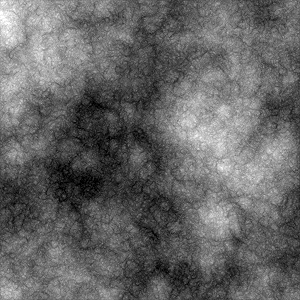Turbulence

The genesis of the frontpiece illustration is mode 0 -turbulence. We base the cost and routing return map on this underlying rendering. As noted in the -plasma tutorial, it is our wont to set a particular seed in G'MIC's random number generator (via srand) so that we can reproduce a particular pattern; what we have here may as well be called "Turbulence Pattern 56712". Mode 0 turbulence employs the abs command as a mixer; at each stage of its development, any zero-crossings are folded back into the positive region, generating numerous discontinuities — creases — both large and small. These emulate rilles and waterways. Being local minima, the rilles have low intensities; when we derive a cost map from this turbulence, rivers or lightning bolts will tend to follow these rilles. We revisit this idea downstream from here. We render the turbulence so that it exhibits large-scale features, develop the pattern through 12 octaves and set a modest decay factor of three between each octave. While large-scale features are present, low-magnitude, small-scale features persist.

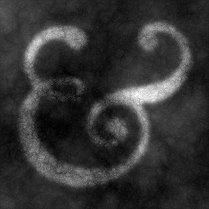Turbulence with Depression

We impress a Goudy 1911 Bookletter ampersand on the cost map. First, we are obsessed with this ampersand (but you knew that). Second, we'd like to steer our lightning bolts so that they roughly trace parts of the ampersand's shape. Since we're playing the Watershed Game, we go about making a general depression in the turbulence in the shape of the ampersand; we blur the ampersand slightly to avoid abrupt drops into the basin. We anticipate that as lightning bolts trace along minimal paths, those will thread through the lower elevation ampersand on the way to the reference point isovalue. Once we have blurred and scaled the ampersand, we multiply it with the original turbulence, giving us the final form of our cost map. Our cost map follows directly from sharpening and squaring operations. Sharpening tends to magnify fine detail, alternately, increasing or decreasing the values of out-of-bound pixels, driving them from the mean value of the image and towards its extremes. Squaring makes expensive (light colored) pixels even more expensive. In the larger scheme of things, we are making a cost map where minimal paths will meander a great deal, as we are creating pits and rises and other obstacles that mitigate against the straightforward progression of minimal paths to isovalues. See the -distance tutorial, which provides further details on how cost maps give rise to the "price" of distances.

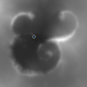Distance to Reference	With a cost map in hand, we harness the -distance command to make the routing return map introduced earlier. To this end, we need an image in which we may take measures of pixel distances to a reference point, so we can then derive costs. Forthwith, then, we conjure a black image from the aether and set a single reference point, a pixel with isovalue one. We plot the reference point at coordinates [400, 430], on the e-loop of the ampersand, an arbitrary choice, but one almost in the center of the image and with just a few distinct approach directions. This input is then included in the -distance command's selection decorator. -distance replaces this input with a distance map. Each pixel in this new map holds the computed distance from that pixel to the reference point. The image of the reference point in the distance map necessarily has a computed distance of zero. All other pixels contain a positive measure, the cost map derived distances to the reference point. Should we care to look at the distance map sideways, pretending, say, to regard the distance measures as heights above a reference level, then the reference point could be seen as being at the bottom of the watershed, with all other points rising in altitude above that. Playful as it may be, this viewpoint has its uses in the Watershed Game.
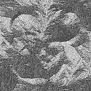Routing Returns at Six Kilometers — Too Small To See!	For our purposes, this distance dataset is only a means toward another end, the routing return map. -distance generates such when in mode 3 or 4. Both modes provide routing return maps and both use Dijkstra Algorithm to find the least expensive path. Their difference is a subtle one. Mode 3 regards two rectangles sharing only one corner has having distinct, disconnected interiors — the low-connectivity setting. Mode 4 regards them as having common, connected interiors — the high-connectivty setting. Neither alternative is "more correct", but each gives rise to different maps. With a routing return map in hand, we can select any pixel as a starting point and plot the least expensive path to the reference point, our nascent lightning bolt.
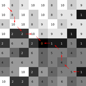Routing Return Detail	The conventional output from -distance is a distance dataset which furnishes point-wise distances of each pixel in the original image to the reference point. For the Great Watershed Game, we use the routing return map instead and throw away the distance dataset; it is not used to make lightning bolts. The routing return map is a point-wise collection of control words, detailed in Walking The Path, one corresponding to each pixel in the distance dataset. Given a pixel, the associated routing return conveys to an imagined cursor the least expensive direction it needs to step in order to move "closer" to the isovalue, in quotes because the routing return may shift the imagined cursor away from the isovalue, at least in terms of Euclidean distance. However, when -distance is furnished with a point-wise cost map, as we have done here, the "shortest distance" is the minimal path with the lowest cost sums, which likely is not the shortest distance by Euclidean measure. On the left, we have schematically reproduced the 9×9 pixel neighborhood around the reference point's image in the routing return map. The numerals represent routing returns, each with three two-bit directional fields that collectively move an imagined cursor away from, or toward the isovalue, along each cardinal direction. Numerals 1, 5, 4, 6, 2, 10, 8 and 9 direct an imagined cursor, respectively, west, northwest, north, northeast, east, southeast, south or sourthwest. The special routing return 0 tells the cursor not to move; once a cursor is given such a directive it necessarily stops; it has been told to go nowhere so can never acquire another directive. The -distance command computes these point-wise routing returns based on the cost map; in aggregate, these routing returns put an imagined cursor at a given point on a minimal path toward the nearest isovalue, one that accumulates the least cost along its length.

Tracing Lightning Bolts

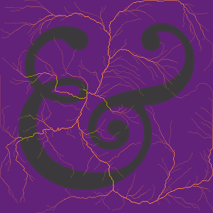Lightning Rendered from Cheap Paths

This brings us to the Watershed Game. The least expensive path from any pixel to the reference point arises from a "step-and-check" procedure. Our "path walker," -paintbolts, is built around a -do … -while block. An outer -repeat loop generates a random number of initial starting points from which we will trace minimal paths to the reference point. An inner -do … -while block traces one such path through a "step-and-check" procedure. Starting from an initial pixel [$kx, $ky], -paintbolts marks its first step on a separate output image. Then, referring to the routing return map for the coding of this pixel, determines its next move. This arises from a parsing of the coded directive, stored in $rdir and implemented through a pair of -if…-elif…-fi chains, one for the x cardinal direction and the other for the y cardinal direction. These two chains determine if there is a forward or reverse step in either cardinal direction. Being a two dimensional walker, -paintbolts has no chain for decoding the ±z cardinal direction. In any case, a non-negative directive will alter either $kx or $ky or both with forward or backward steps. Now on a new pixel, -paintbolts marks a new step and refers to the routing return map for the coding of the new pixel. And so on. And so forth. Eventually, if -distance created a sane routing return map, $rdir will obtain a zero value, which is the directive that translates to "No further steps." The path walker has arrived at the reference point and -paintbolts drops out of the -do … -while block, now to pick up a subsequent initial point for a new lightning bolt, should there be any left. Because of turbulence in the cost map, the least expensive path will be locally jagged, but it will converge on the reference pixel on a larger scale in a lightning bolt kind of way. You will note that one path is only faintly drawn, but many such paths will converge on the reference point from only a few directions and overlay one another to a considerable extent. The overlaid portions will seem very bright in the final rendering, as many paths contribute to the brightness. In aggregate, these paths will look like lightning bolts striking a common point.

Command Reference

Updated: March 07, 2023 21:23 UTC Commit: 220bd6b91cf3556158551b6ca6d8f6e242b72850