K-Means

Dover's Hill progressively decimated, near Chipping Campden, Gloucestershire, The Cotswold, UK James Trickey Wikimedia Commons

K-means finds the dominant colors in an image through an iterative corrective process. In practice, users specify the number of colors as a parameter, often without any reference whatsoever to the statistical properties of the image. They have the desire (or are constrained because of technical reasons) to reproduce an image using a fixed (and usually small) number of colors. They can choose the colors, and want to choose the best ones. K-means will find quite good ones, but finding the "best" is currently an outstanding research problem.

Users might provide a palette of colors as initial hints. The hints could be quite good or really bad; the k-means algorithm (almost!) always converges to a good solution, and (almost!) always better than any hints that users may have provided beforehand. Bad hints just take longer — maybe a lot longer — to converge. As used in the G'MIC -colormap command, the k-means algorithm gets pretty good hints from an initial run of the median-cut algorithm.

The best way to approach the K-means algorithm is to think of colors as points in a color space where the notion of “dominant color” translates into a cloud of color points clustering, more or less closely, around some mean: a dominant color.

At the outset, K-Means has no idea where these may be, but, taking the initial palette as so many starting points, the algorithm “tags” each color in the image with the ID of the closest palette color (see -index). This tagging process is sometimes called the assignment phase. These separate groups of colors, each with a tag in common, are initially the best known clusters to the algorithm.

How good are they? To find out, the k-means algorithm locates the median color of each cluster. This median, the "center of the cluster," is taken to be the weighted average of all similarly tagged colors. The algorithm weighs a particular color by the count of its appearances in the cluster divided by the total count of all colors in the cluster. This weight, a ratio somewhere between zero and one inclusive, is the relative size of a particular color population with respect to the whole. This scheme ensures that particular colors contribute to the hue of the mean color only in relation to their numbers as a fraction of the whole. Computing these weighted averages is sometimes called the update phase. 

The algorithm takes the difference between all weighted averages, one for each swatch in the color palette, and the original color swatches. If average magnitude of these differences exceeds a certain predefined tolerance, then the algorithm takes the weighted averages as the better solution and cycles using these as entries in the updated palette. The process completes when two successive palettes are found to be identical, or so similar that their differences do not matter.

1. Begin with an original image, a minimum error threshold, ε, and a palette₀, with k swatches indexed {0, …, k – 1}. Let palette ₀ be the “current palette,” to wit:

   palette _C←palette ₀

2. Tag each pixel in the original image with the index of the most closely matching swatch in the current palette _C, producing an intermediary image where every pixel is a two-field record of integers containing the actual hue in the least significant field and the closest matching swatch index in the most significant field.

3. For each swatch index i in palette _C with index i in {0, …, k – 1}:

   1. Generate per-channel histograms with 2^d bins from all pixels tagged with swatch index i. d is the bit depth of the channels; 2^d for d = 8 bits/channel is equal to 256 histogram bins.

   2. For each histogram bin, multiply its count with the corresponding luminance value from a black-to-white ramp of 2^d steps. For each channel, this step selects luminance values from the ramp observed in the image and associated with swatch i. Luminance values that have not been observed with swatch i's tag necessarily have zero counts while those with positive counts have been tabulated in direct proportion to their frequency of appearance.

   3. Normalize the products of counts and luminance values through dividing by the total count of pixels associated wih the swatch, yielding weights for each color relative to the whole swatch population. The sum of these variously weighted colors is the weighted average color of swatch i.

   4. Subtract this weighted average color from the one in the current palette. This difference measures the offset from the median recorded in palette _C and the updated median tabulated from the image.

4. Take the average of the absolute values of all k differences computed in step 3d and compare with ε.

5. If this average of absolute differences exceeds ε, define palette _C+1 based on the weighted average colors found in step 3c and continue with step 2 using palette _C+1.

6. Otherwise, accept palette _C as an optimized version of the initial palette ₀

Step 2 implements an assignment phase. For each image pixel, the algorithm determines which swatch is nearest to the pixel in color space distance and assigns the swatch ID to that pixel. This task is implemented almost entirely by the G'MIC -index command. Through this process, the algorithm can readily group image pixels by swatch ID.

The computation of new averages in steps 3b and 3c initiates an update phase. If image pixels group with the same swatches for two successive palettes, then counts do not change and the averaging in step 3c produces the same set of median luminance values. This completes the algorithm, furnishing a corrected palette.

On the other hand, if, in successive palettes, different pixel groupings arise then counts change, as one re-tagged pixel affects two counts, two averages and two swatches. In this case, an updated palette with shifted medians arises.

The trial then recommences with this updated palette, necessary because in computing new averages, cluster medians move – and almost certainly, in their new locations, some pixels which used to be rather closer to one median are now rather closer to another, creating new misalignments.

The heuristic belief is that these misalignments become fewer in number as iterations proceed. That is, medians eventually migrate to the center of their “true” clusters giving rise to a minimum of misalignments and updates that barely change in successive rounds.

m={im} M={iM} -normalize. 0,255 <color mapping and tagging> -do <k-means iteration> -while {$diff>0.5} <Convert back to original colors>

Normalization

Our detail k-means walk through concerns itself with a single-channel gray scale; concepts here extend without change to multichannel images – it is the same story repeated for however many channels an image may have.

We begin with a pair of math expressions capturing the initial minimum and maximum values of the original image, followed by a temporary normalization of the image to the full luminance range of 0,...2^d – 1. No generality is lost in normalizing an image to the full luminance range of the bit depth of the channel. Its geometric effect in RGB color space is one of magnifying distances, but the relative positions of pixels with respect to their neighbors or their cluster medians do not change. This normalization step is necessary to make full use of the luminance range of the histograms introduced in step 3a. Without normalization, nearly all pixels of an extremely subtle, low-contrast, gray-on-gray image wind up in just a very few bins of the histogram and we would be unable to fully resolve clusters. At the end of the run, we apply m and M in a renormalization step to scale the swatches of the palette back to the luminance range of the original image.

Illustration 1

<normalization> --colormap $1 --index.. [-1],0,0 -+[-3,-1] -do <k-means iteration> -while {$diff>0.5} <Convert back to original colors>

Color Mapping and Tagging

The first step of great moment is the running of the gradient-cut algorithm on the renormalized image; this produces an initial trial palette which the k-means algorithm refines.

Recall that -_colormap is a “private” G'MIC command encapsulating the median-cut algorithm, so on the second line of our code excerpt, everything documented in Median-cut happens and, with its left-hand decoration written as a double-hyphen, the -_colormap command returns leaving the original image intact and the initial palette following it on the image list. Note that $1 is a substitution sequence for the first item on the command line, in this example, an argument setting the palette size to 4 color swatches, each corresponding to a (presumed) cluster median in the original image, at least in the humble opinion of the gradient-cut algorithm.

Illustration 1 depicts the initial case. The dark blue markers illustrate the luminance distribution of values in one channel of the original image. There seems to be local peaks – lots of pixels with the same luminance – at values of 0 (about 50 pixels), 88, (about 15 pixels) 150 (about 30 pixels) and 255 (about 108 pixels). Potentially, these peaks are at or near the median values of clusters occurring in this channel. All other luminance values have just single digit counts and many luminance values have zero counts, corresponding to no pixels at all.

Four very colorful markers are superimposed on this luminance distribution. For this particular channel, they flag the luminance values within the four swatches of the initial palette. If the swatches truly align with the median values native to the channel then there would be only small differences between the palette values and those computed in an initial round of the k-means algorithm. However, the values of these swatches, 119, 147, 168 and 202, seem quite far from some of the peaks in the distribution, particularly those at either end of the distribution.

Illustration 2: Image channel, dimensioned to a one pixel row ([0]), and the presumed optimum palette ([1]). Only one channel is depicted.

<normalization> --_colormap $1 --index.. [-1],0,0 -*. 256 -+[-3,-1] -do <k-means iteration> -while {$diff>0.5} <Convert back to original colors>

This situates us at Step 1 of the k-means algorithm. The pixels of the original image, still arrayed in one row, is in position [0] and the initial palette follows it at position [1]; see Illustration 2. The error threshold, ε is hard-coded at 0.5.^*

--index associates each pixel in the original image with the closest of the four swatches from the palette, commencing the assignment phase of Step 2. Its particular arguments disable dithering, which serves no purpose here, and requests an index map. The output pixel is not colored with the chosen palette swatch, but has the index number of the closest swatch instead. These are the tags which later commands assign to image pixels.

The “closeness” of a pixel color and a palette swatch is grounded on the idea that color may be thought to occupy a three dimensional color space, where the additive primaries of red, green and blue occupy analogous roles to the x, y and z coordinates of the volume around us. One need not go into the math to find sympathy with the idea that blue-green and cyan must be very close together, but a substantial distance from red or orange. Assigning the primaries to coordinate axes lends rigor to this notion; we can then use a metric relationship like the Pythagorean Formula to calculate precisely the distance between two colors.

The next two steps complete the “tagging” of the assignment phase. -* scales the tags by 2^d (256 for eight bit deep channels) and -+[-3,-1] combines the tags with the pixels, in effect turning each into a two-field record: the most significant field has the tag, the swatch index of the closest palette color to the pixel, and the least significant field has the actual value. In a sort, such as what -histogram does, this particular arrangement causes pixels to group first by swatch assignment, and next by intensity value, effectively grouping image pixels into swatch-specific histograms. The utility of this becomes manifest in the next section, covering the update phase.

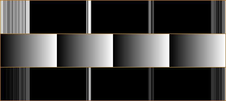
Illustration 3: The top row is effectively a series of four histograms, one for each swatch. Each pixel represents a histogram bin containing a count of pixels tagged with a particular swatch ID and having a particular luminance value. These bins are sorted first by swatch ID, then by counts for particular luminance values. Middle: one ramp for each swatch ID. Ramp steps are multiplied pixel-wise with the top row histogram bins to produce the bottom row, luminance values weighted by histogram counts. The average of these weighted values is that which should be associated with the swatch ID, based as it is on actual population assessments. Of course, these averages may differ from those comprising the current palette.

<normalization> <color mapping and tagging> -do -repeat {s} -shared[0] $> --histogram. {$1*256},0,{$1*256-1} -remove.. -input.. 256,1,1,1,'x' -resize.. {w},1,1,1,0,2 -mul.. [-1] -resize[-2,-1] $1,1,1,1,2 -max. 0.01 -div[-2,-1] -done <difference testing> -while {$diff>0.5} <Convert back to original colors>

K-Means Iteration

The tagging in Step 2 of the algorithm makes possible a sorting of image pixels first by swatch ID and then by counts of luminance value, grouping into one set all the pixels that -index deemed as being close to a particular swatch. The aim of Step 3 in all its parts, a – d, is to determine if the average value of these pixels in each swatch grouping differs significantly from that of the swatch. If it does, then the swatch needs updating.

The G'MIC implementation flattens the per-swatch iteration given in the k-mean overview. The sorting, first by tags and then by value, essentially generates as many histograms as there are tags. These can be processed in parallel in one image, as shown in Illustration 3. The G'MIC implementation just iterates over image channels, and carries out Steps 3a – 3d in parallel through the ganged-together images shown in Illustration 3.

Computing the average luminance value of a collection of pixels tagged with the same swatch ID takes place in the -repeat {s}…-done block, producing, in each loop over a channel, a set of averages, one for each swatch. It suffices for us to follow the evaluation of one channel.

-shared[0] $> places a virtual image on the end of the list containing the current channel to be processed, this identified by the substitution symbol $>, which successively selects channel 0 through n, n being however many channels an image may have. --histogram. {$1*256},0,{$1*256-1} essentially generates a series of 256 bin histograms, one histogram for each unique swatch ID, this by virtue of the tagging done in Step 2. Note the double-hyphen left-hand decoration on --histogram. It operates on a shared buffer belonging to the original image and without such notation it would have replaced one channel of the original image, breaking it. The double-hyphen form has copy semantics, so the original is left alone.

Note also that $1 is the substitution symbol for the number of swatches first requested by the user, the product $1*256 ensures that the histogram will have sufficient bins to accommodate every possible swatchID/luminance value pair. The value range given by the second and third parameters, 0,{$1*256-1} sets the range to an extent so that every possible product of swatch ID and luminance value will just map to just one and only one bin. Finally, -remove.. takes the virtual image off the list. Of course, no bytes are really lost by virtue of its virtuality – the buffer still exists a component of the original image, but is no longer shared. In this case, -remove is '-unshare', by another name.

The result of this command is the histogram at the top of Illustration 3. Strictly speaking, it is one histogram, but each 256 bin section can be regarded as a distinct histogram for all pixels tagged with a particular swatch ID. Each bin tabulates how many pixels of a specific luminance value contributes to a particular swatch ID. If the luminance value associated with this swatch ID is (more-or-less) correct, then the pixels that are more-or-less like its value have high counts, and others, less like the swatch, have low or zero counts. This may not be the case when the value of the swatch isn't really much like the pixels tagged with its swatch ID. This will give rise to an average value for the swatch that differs from the value associated with it, as will be seen in later steps.

-input.. 256,1,1,1,'x' creates a 256 step ramp. -resize..{w},1,1,1,0,2 combines the 'no interpolation' resizing parameter (0) with the cyclic boundary policy (2) to rubber-stamp the ramp along the width axis, a neat trick. Fortuitously, each ramp step aligns with its counterpart tabulation and the product of the tabulation and ramp values, obtained with -mul.. [-1], results in a weighted value, essentially a luminance value scaled by the number of times it has been 'observed' as being tagged by the swatch ID. This datum, in conjunction with the other 255 count × ramp value multiplications, can be summed together to find the weighted average luminance value produced by all the pixels tagged with a particular swatch ID.

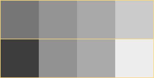Illustration 4: The top row is the palette that -index used to group pixels by swatch IDs. The bottom row has the average luminance values found those groups by one iteration of the k-means algorithm. The difference indicates that the initial palette wasn't exactly correct.

<normalization> <color mapping and tagging> -do -repeat {s} -shared[0] $> --histogram. {$1*256},0,{$1*256-1} -remove.. -input.. 256,1,1,1,'x' -resize.. {w},1,1,1,0,2 -mul.. [-1] -resize[-2,-1] $1,1,1,1,2 -max. 0.01 -div[-2,-1] -done <difference testing> -while {$diff>0.5} <Convert back to original colors>

-resize[-2,-1] $1,1,1,1,2 may not seem to be an averaging tool, but resizing the width of the histogram to just the number of swatches in the palette, in conjunction with the linear interpolation parameter (1) essentially averages each 256 block of luminance values × counts into one pixel containing the average product of luminance values × counts. So each pixel in the penultimate image on the list [-2] contains this quantity:

$$\frac{\underset{k=0}{\overset{255}{\Sigma ˆ‘}}{v}_k{c}_k}{256}$$

for each swatch.

Alas, this is not quite the weighted sum of luminance values that we want; weights should partition unity, that is, the weights should look like percentages which together add up to 100% because we are adding up fractional parts of a whole. But the weights here are just the raw counts, which add up to some total count, so our results are fantabulously skewed. Fortituously, the piece we need to turn this expression into a proper weighted sum of luminance values can be had from the last image on the list, the histogram counts c_k for each luminance value v_k of pixels. Both the penultimate and the last image on the list was a part of -resize's selection, so each pixel in the last image on the list [-1] is:

$$\frac{\underset{k=0}{\overset{255}{\Sigma ˆ‘}}{c}_k}{256}$$

for each swatch. So we can be almost home free by just performing a pixel-wise division of the penultimate image (averaged luminance values × counts per swatch) by the last image (averaged counts per swatch), which is what -div[-2,-1] does in far less time than it takes to write about it.

$$\left(\frac{256}{\underset{k=0}{\overset{255}{\Sigma ˆ‘}}{c}_k}\right)\times —\left(\frac{\underset{k=0}{\overset{255}{\Sigma ˆ‘}}{v}_k{c}_k}{256}\right)\to ‡’\frac{\underset{k=0}{\overset{255}{\Sigma ˆ‘}}{v}_k{c}_k}{\underset{k=0}{\overset{255}{\Sigma ˆ‘}}{c}_k}\to ‡\underset{k=0}{\overset{255}{\Sigma ˆ‘}}{v}_k\frac{c_k}{{\mathrm{\Sigma }}_c}\mathit{ where }\underset{k=0}{\overset{255}{\Sigma ˆ‘}}{c}_k={\mathrm{\Sigma }}_c$$

The right end of the simplification tells us to scale each pixel value v_k by the ratio of its count, that is, the frequency of occurence of the value v_k tagged with a particular swatch ID, and the total count of all pixels tagged by that particular swatch ID. These fractional weights by themselves add up to one, or 100%, or unity, so all of the terms $v_k\frac{c_k}{{\mathrm{\Sigma }}_c}$ sum to a luminance value that is not magnified or diminished by inadvertant scaling factors.

The only little bit that keeps us shy of being home free is the possibility of a count average being zero, which would induce a division by zero which would blow everything up and possibly get people annoyed with us. To avoid this calamity, -max. 0.01 visits every pixel in the image of averaged pixel counts and should that command find a zero count, it replaces it with 0.01. That is, every averaged count is left alone unless it is zero, when it gets enough of smidgin value to keep the math library at peace with the world.

This leaves us at Step 3c, a new palette of average, per-swatch values, based on the pixel-tagging performed by -index. Illustration 4 compares the current and new palettes at the end of the first iteration, suggesting quite a difference betwixt the two.

Illustration 5: (Compare also with Illustration 6), superimposed over the histogram of a channel of the original image are the channel values of swatches of successive palettes, converging toward a solution. Iterations read from bottom to top; the initial palette is at the bottom, marked with iteration 0, the solution appears at the top, occurring 25 iterations later. Vertical lines descending from the plots locate the swatches in the histogram. The dark end of the histogram and the darkest swatches are on the left, the lightest on the right. To a lesser and greater extent, the two lightest swatches seemed initially to converge on a light solution, then, around iteration 9, switch directions and commenced converging on a darker solution, reaching it sixteen iterations later.

<normalization> <color mapping and tagging> -repeat {s} <Compute swatch averages> -done -append[2--1] c -sub.. [-1] -abs.. diff={{-2,is}/w} -rm.. -and.. 255 --index.. [-1],0,0 -mul. 256 -add[-3,-1] -while {$diff>0.5}

Differencing the Averages and Comparing Palettes

In the sweet fullness of time, the k-means iteration processes all the channels of an image, leaving on the image list, from position [2] to the end, a series of gray scales that constitute the channels of the newly estimated palette. Position [0] has the tagged pixels of the original image, still arrayed along one row, and position [1] has the current palette, which may or may not be significantly different from the just-estimated palette. This situates us at Step 5 of the algorithm, the decision point.

-append[2--1] c assembles the series of gray scales into a multichannel palette. Superficially, it may seem to be little different to the current palette in position [1], but appearances can be deceiving. The -sub.. [-1] command effectively replaces the current palette with the differences between it and the newly estimated palette. The -abs.. command follows, converting positive and negative differences to positive differences, because it is the cumulative magnitudes of change that matter to us, and not the direction of change. The diff={{-2,is}/w} command performs the accumulation, assigning the average cumulative differences to $diff. G'MIC maintains the sum of pixel values of an image as a property, is, and the math expression {-2,is} assesses this property from the penultimate image, second from the last, and the average is taken by dividing it by the width of the last image.

A purist may have written the average difference calculation as diff={{-2,is}/{-2,w}} obtaining both properties from the same image, but the newly estimated palette and the image of swatch differences have the same dimensions, so an economy of keystrokes trumps a purity of expression. So there. Get over it.

Everything following is setup for the next iteration, though such may not take place. -rm.. cleans the differences image off the image list, and -and.. 255 strips the now-outdated tags from pixels in the original image. Note that 255 as a binary mask which admits the least significant eight bits, the pixel luminance values, but zeros out the swatch ID tags, now outdated.

The last three steps before the bottom of the -do … -while loop, --index.. [-1],0,0; -mul. 256; and -add [-3,-1] have been dissected already; these implement Step 2, the assignment and tagging step of the k-means algorithm, again done in anticipation of another iteration. Whether such actually takes place depends on the boolean expression associated with the -while {$diff>0.5}. If the test succeeds, the average differences across all the channels exceeds the tolerance value of 0.5 and another round of the k-means algorithm occurs. Otherwise, the two last successive palettes are essentially identical, with very, very little to be gained through further iterations.

Illustration 6: Differences of successive palettes, beginning with the not especially well matching palette from the start of the walk through. Convergence of the k-means algorithm is almost always certain, but not necessarily steady and sometimes exhibiting a kind of damped oscillation between two solutions. Here, with our palette, differences dropped exponentially in five iterations from a high of nearly 25 to a low of about 0.6 – and then became stuck for five more iterations, actually losing ground. It broke through to a new solution at the tenth iteration and converged slowly and steadily for the next fifteen steps.

<normalization> <color mapping and tagging> -do <k-means iteration> -while {$diff>0.5} -rm.. -*. {($M-$m)/255} -+. $m

Illustrations 5 and 6 let us step back and see how our initially conjured palette converges onto a solution. Illustration 5 shows the rake's progress of comparable channels of the four palette swatches, superimposed over the histogram first shown in Illustration 1. It diagrams how the values of the swatches changed and converged toward more likely medians over the course of 25 iterations of the k-median algorithm. Read the iterations from bottom to top. Vertical lines dropping from each median locate its place in the histogram.

Illustration 6 shows the convergence toward zero of the average differences between successive palettes. Differences dropped exponentially in the first five iterations, promising a ready solution, then began getting worse from the 6^th to the 10^th iteration. A solution seemed to break at this juncture, and differences between successive palettes steadily converged to zero at the 25^th iteration.